Quarto 📖

MATH/COSC 3570 Introduction to Data Science

Dr. Cheng-Han Yu
Department of Mathematical and Statistical Sciences
Marquette University

Hello Quarto

Why Quarto is a Amazing Tool for Data Science Basic syntax: Markdown and Code

• Last time we learned git and github to version control our documents.

• You first grab hw0 from github, and load it into Rstudio as a project. In the document hw0, you actually opened an Quarto file, right, you make changes, revise it and keep track of your changes by making commits. Then finally you send your updated version of document back to github, so that the version locally in your computer is synchronized with the one in your github. right?

• Today we are going to talk about Quarto, the one you opened last time.

• I’ll introduce some basic stuff, and you’ll learn how to generate a beautiful html or PDF report that includes code, tables, figures generated by the code all together.

• And each of your homework sets will be a qmd file. That’s why I talk about Quarto before we actually touch data and do data analysis.

• Let’s learn this great tool together!

Sharing Data Science Products using Quarto

• Remember that in DS, our ultimate goal is share our data science outputs and communicate with others.
• Today, we are going to learn Quarto that is an amazing tool for generating various different kinds of data science output.

What and Why – Full Reproducibility

• [What] data science publishing system
• Use a single Quarto file (.qmd) to
  • weave together narrative text and code
  • produce elegantly formatted outputs: word/pdf, webpages, blogs, books, etc.
• [Why] Fully reproducible reports
  • Have code, results, and text in the same document
  • Results are generated from the source code, and your documents are automatically updated if your data or code changed.

• WHAT
• Remember in the last stage of DS, we need to communicate our DS results with others.
• qmd is a very useful communication tool that integrates prose/words, code, and analysis results.
• WHY
• Results are generated from the source code, and your documents are automatically updated if your data changed.
• So if your data or code changed, or you need to redo your analysis or rerun your algorithm, you don’t need to actually redo your analysis and copy all of your numbers, tables and figures generated from your code and paste them manually to your Word or Powerpoint file.
• Since your code, results, and text are all in one qmd file, if your data change, your results will be automatically updated with that change. No more copy and paste.
• This greatly saves lots of time. Also, it reduces the chance of making mistakes of copying and pasting, and increases reproducibility of your study, meaning that your code can produce exactly the same result shown in your document.
• Literate Programming

I found an error in the data and added two more cases. Find the attached the modified excel. Can you redo the analysis? - Excel to R - Re-Make the graphs and re-run all the analysis - Copy and paste every updated output from R to your document This is an non-reproducible way fo doing data science.

But there is another way, a better way, a reproducible way.

Why Quarto – Various Types of Output

• Support dozens of static and dynamic/interactive output formats!

• One more reason to use Quarto is qmd can generate various types of output!
• It can produce a PDF, blog, HTML. It can generate slides, website, dashboard, word document, e-books. You name it!
• So once you learn this Rmarkdown, you can prepare any type of output you want for different purposes. You can prepare a paper for submitting it to a journal, prepare slides for your presentation, prepare a website/dashboard for data science results.
• It’s really handy! In fact, the slides I make for this course are all qmd files.

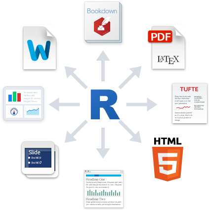
Moving Between Formats Straightforward

HTML Document

{{}} datascience.qmd

title: "Data Science"
format: html

Presentation Slides

{{}} datascience.qmd

title: "Data Science"
format: revealjs

Website

{{}} _quarto.yml

project:
  type: website

website: 
  navbar: 
    left:
      - datascience.qmd

–> a lesson in document form
–> the same content in presentation form
–> the same content on a page in a website,

and you can see that all that needed to change going between these formats is a few lines in the yaml. Nothing in the content part of my document. No slide breaks to remove, no citation style to change, no headings to re-level. This ease of transition has freed up time to focus my time on content, and that, folks, is the dream!

Why Quarto¹ – Integrate Multiple Languages

1. Quarto is actually a command line interface that can render .qmd files into different output formats using commands in terminal.

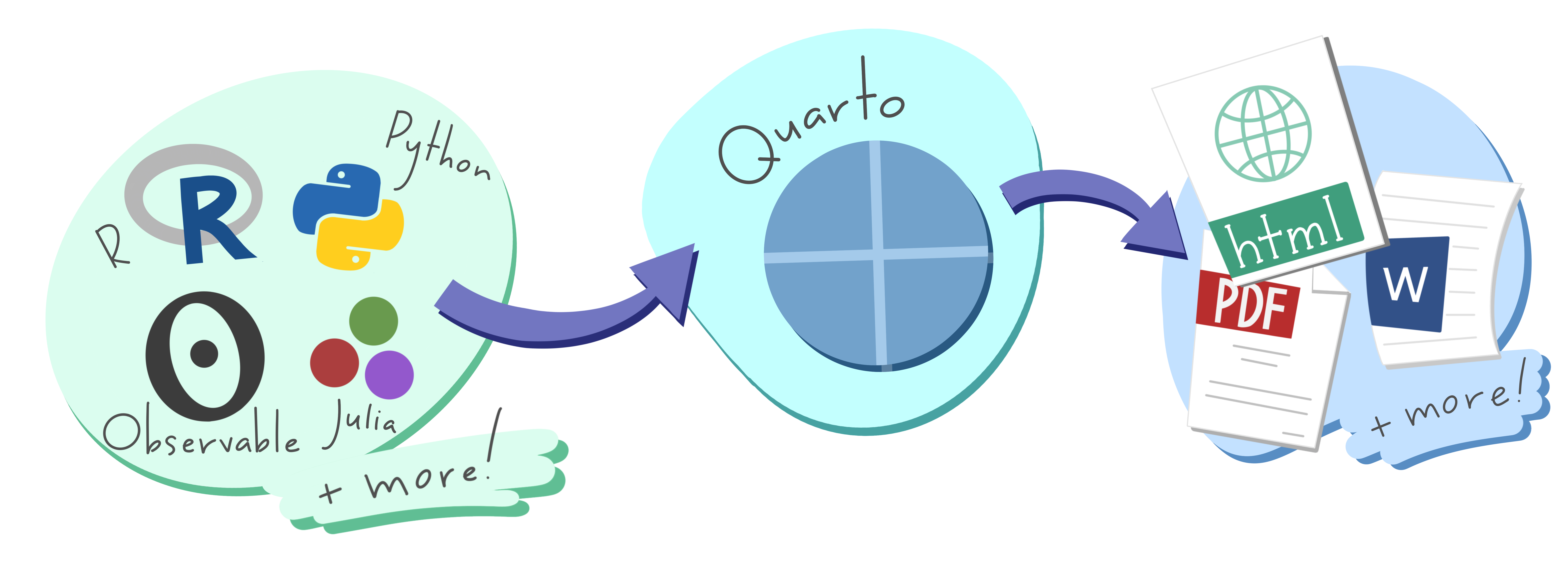
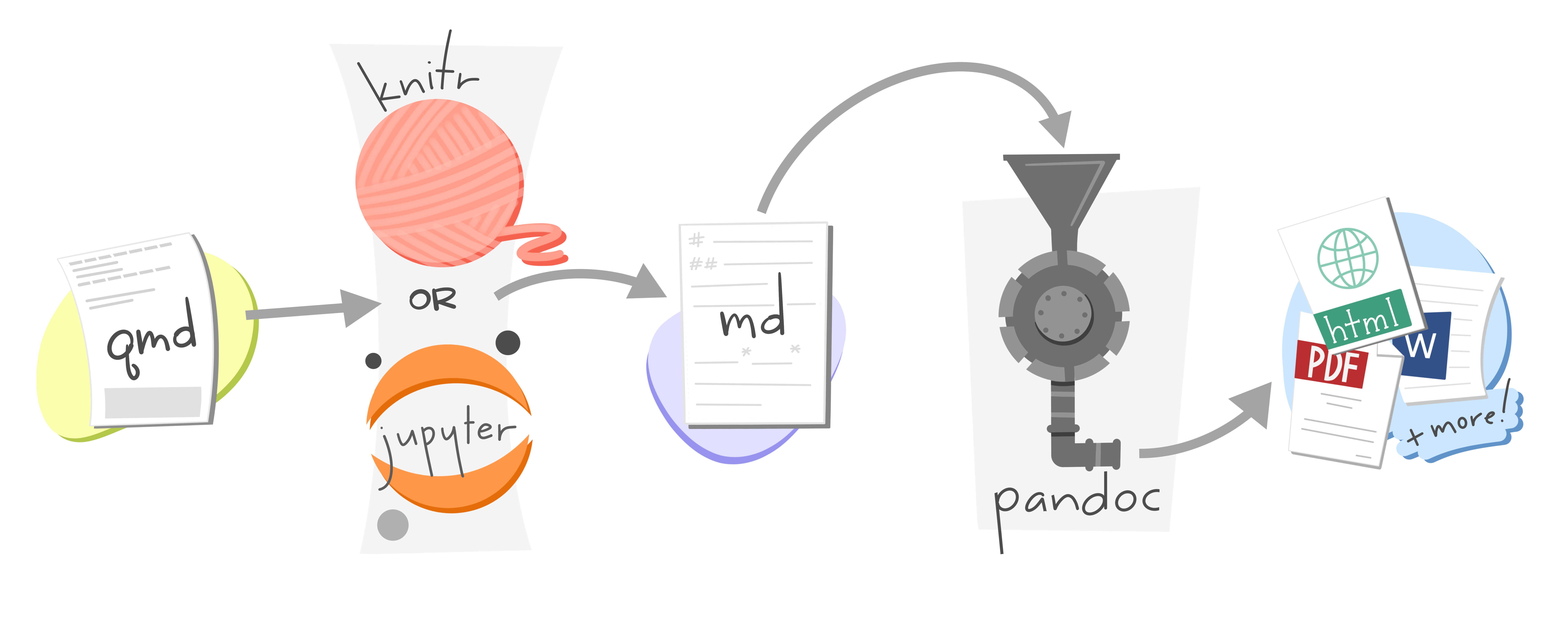
Quarto Is Built on Pandoc

• R uses knitr and Python/Julia uses Jupyter to evaluate our code and turn qmd into md file.

• So what does Quarto do so amazingly for us?
• When we hit Knit, your qmd first uses the knitr package to execute and translate our code, and then creates a new markdown document which includes the code and its output.
• The markdown file is then processed by a document converter called pandoc which is responsible for creating various document format you like.
• The entire process looks and sounds complicated, and indeed it’s complicated. But qmd makes it simple. All we need is to click on the Knit button, and qmd does everything for us.

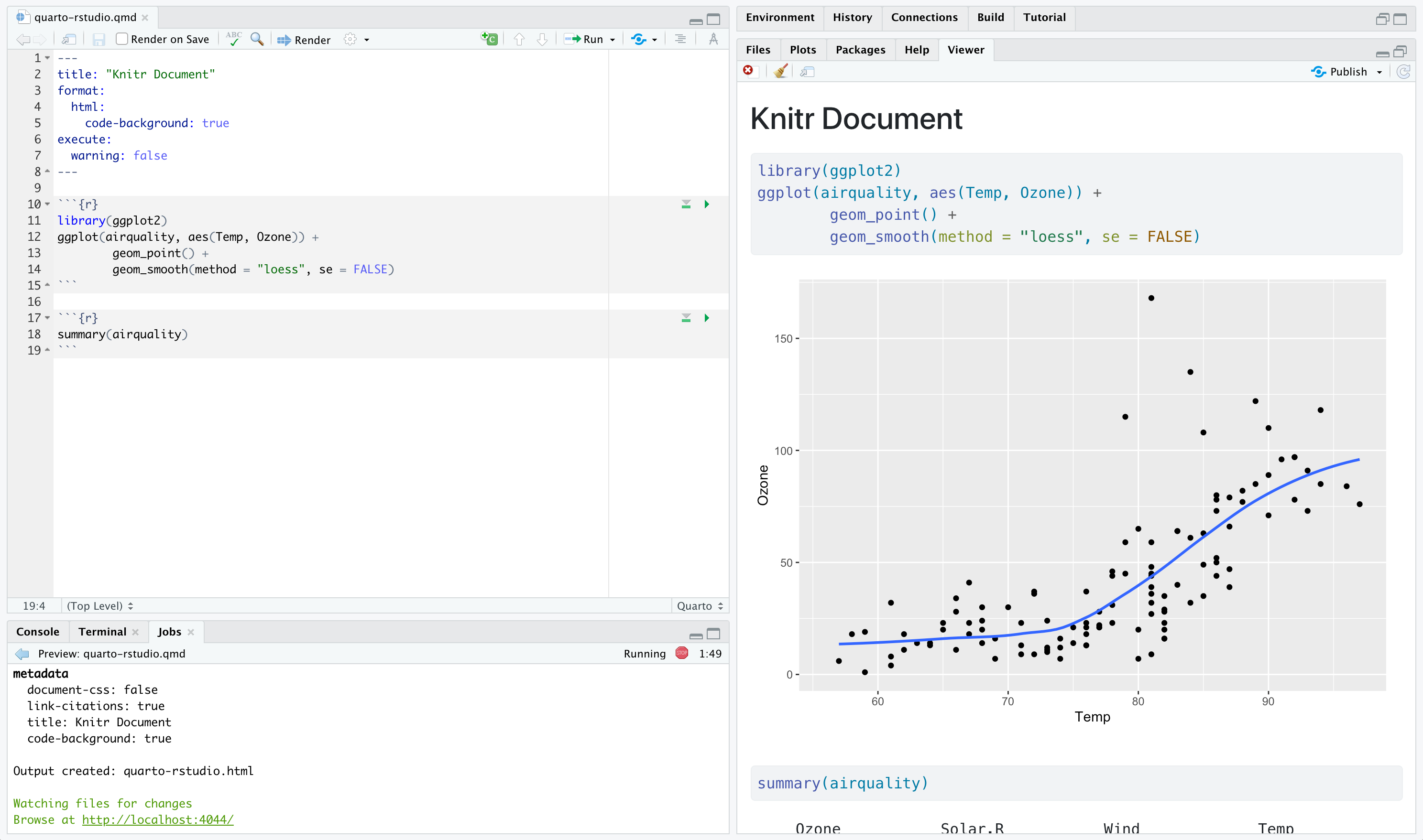
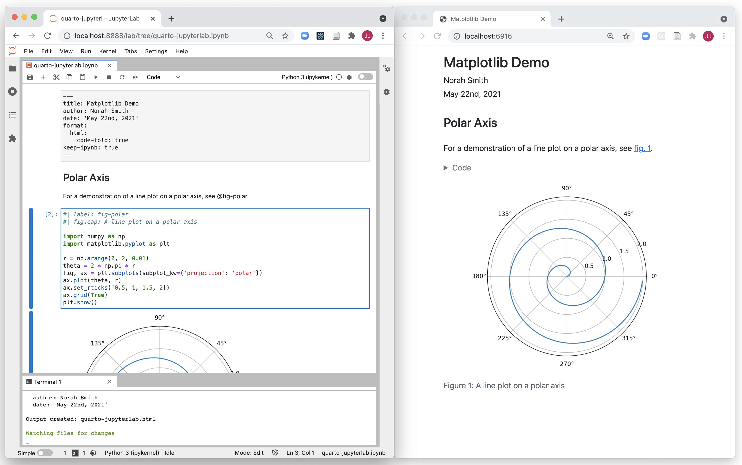
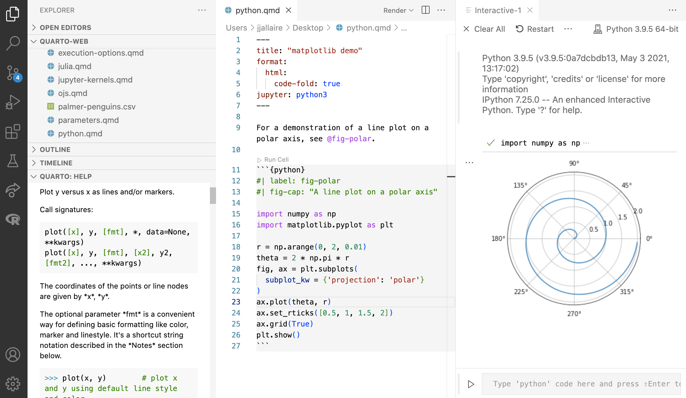
Why Quarto – Comfort of Your Own Workspace

Why Quarto – Simple Markdown Syntax for Text

To generate a PDF report, you prefer writing this with 24 lines…

• Another reason to use Quarto is that its syntax is simple.
• We can generate this PDF report including code and figures using this concise qmd file on the right.

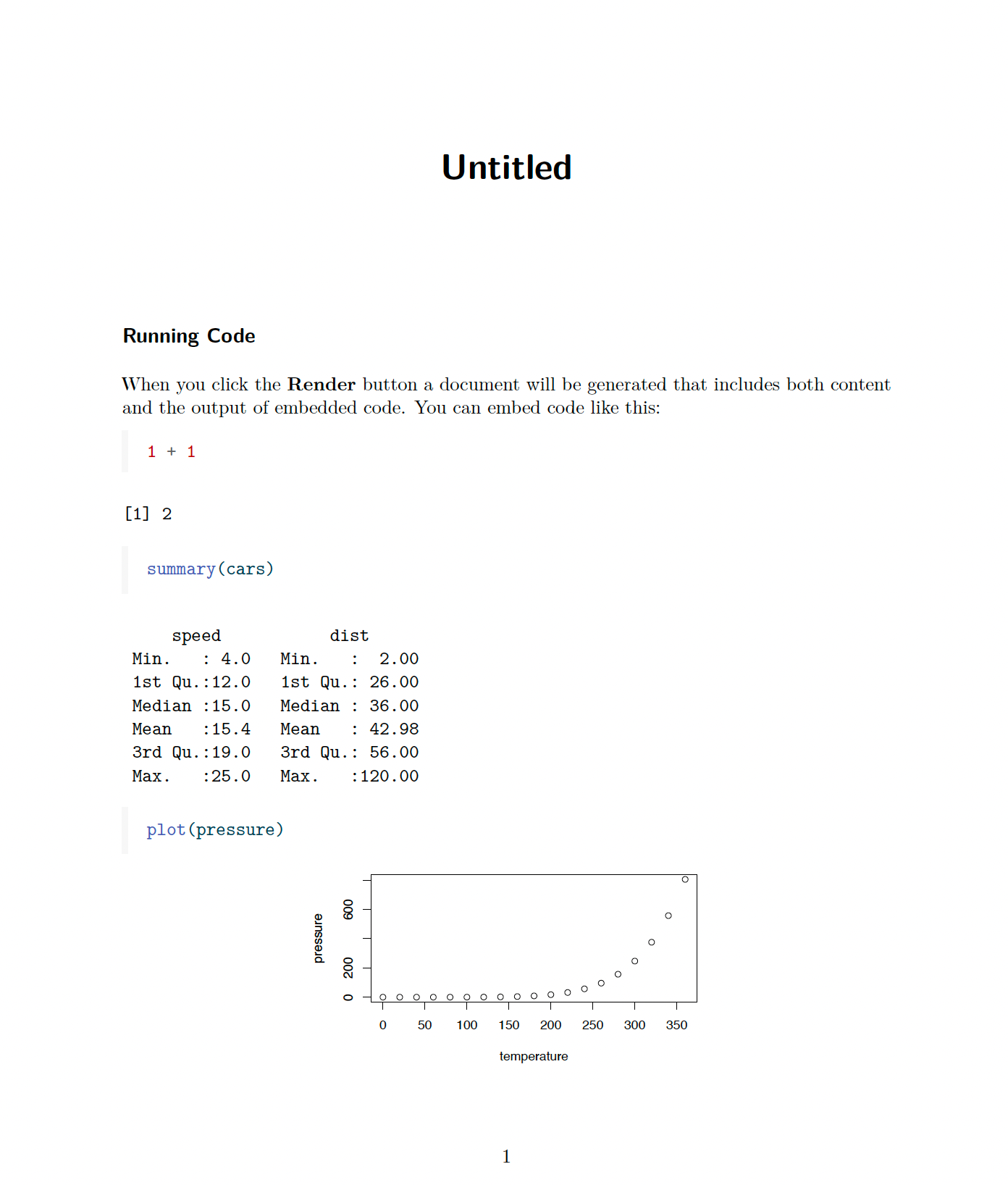
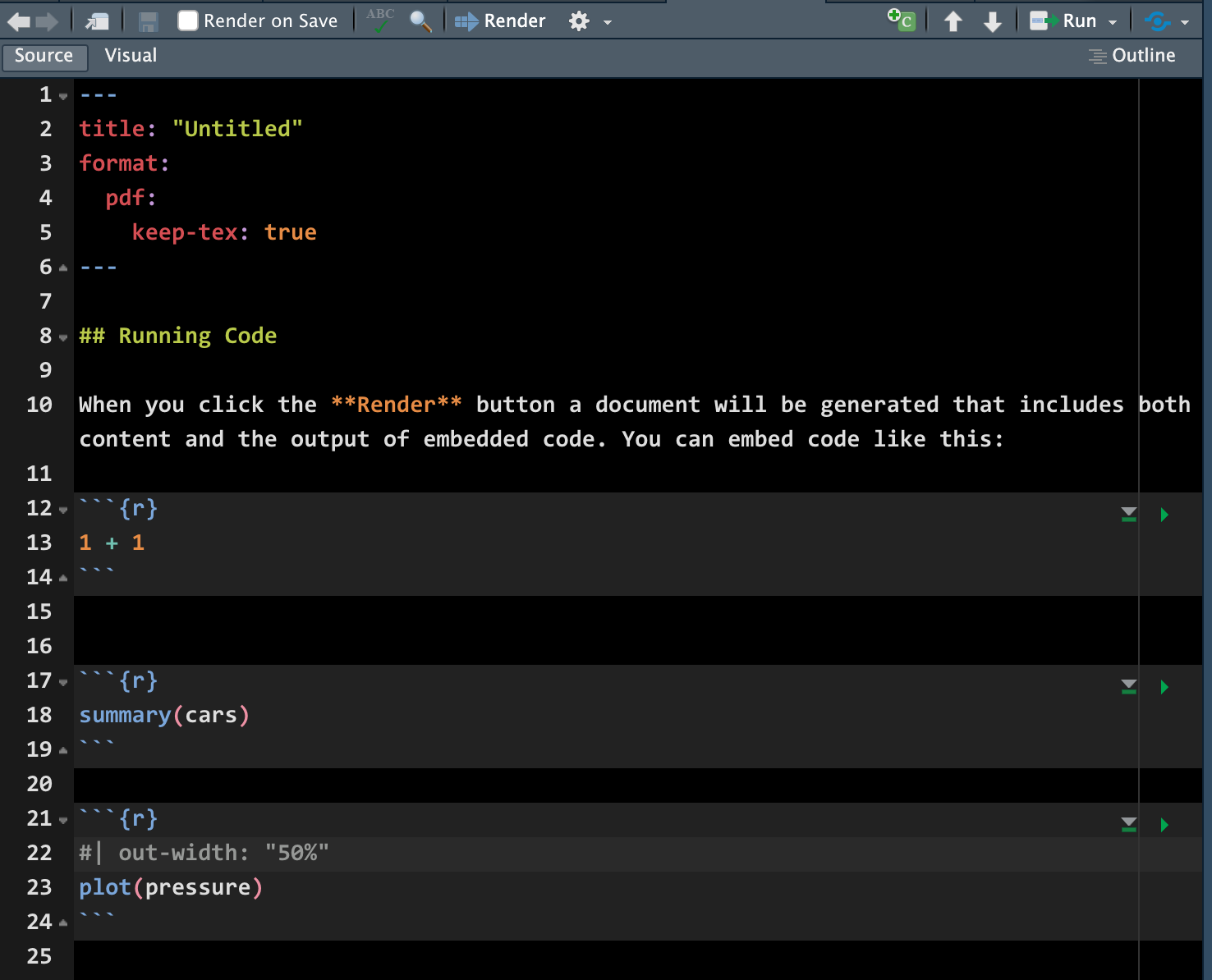
Why Quarto – Simple Markdown Syntax for Text

Or this with 250 lines!?

• We can also generate the same PDF report using this document processing format.
• Which one you prefer?
• Does anyone know what tool is used for generating the PDF? It’s called LaTex.
• You can see the qmd file is cleaner and much more concise.

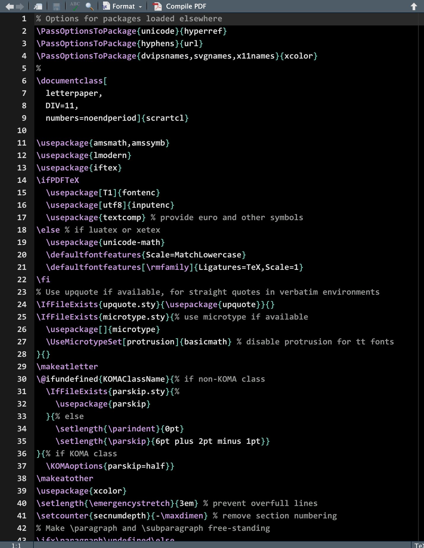
Markdown

• Quarto is based on markdown, a markup language that is widely used to generate HTML pages.
• Markdown is a lightweight and easy-to-use syntax for styling the writing on the GitHub platform.
• We go through basic (Pandoc’s) Markdown syntax together, and you can learn more at:
  • Markdown Tutorial
  • Mastering Markdown GitHub Guides
  • Markdown Guide

• In my opinion, comparing to HTML, Markdown format is more friendly and easier to learn.

Quarto file = plain text file with extension .qmd

---
title: "ggplot2 demo"
date: "1/25/2024"
format: html
---

## Cars
There is a relationship between *miles per gallon* and *displacement*.

```{r}
mpg |> ggplot(aes(x = displ, y = hwy)) + 
  geom_point()
```

YAML Header (“YAML Ain’t Markup Language”)

---
key: value
---

• The first part is the YAML header, which is surrounded by a pair of three dashes.
• YAML is a human readable language that is commonly used in configuration files of programs.
• Here, YAML header defines metadata of the document, for example, title, date, and output format.

Markdown Text

• The second part is text.
• And as we’ve discussed, the syntax for text is Markdown. We’ll learn some basic syntax later.

Code Chunk

```{r}
## code right here
```

• The third main part of a qmd document is the so-called code chunk. which is surrounded by a pair of three backticks.
• The code written in code chunks will be run once you compile your qmd file, and any output generated by your code will be printed out in the final document. All right!
• Any questions

02-Quarto File

• Go to your GitHub repo lab-yourusername. Clone it to your Posit Cloud as a project in 2024-Spring-Math-3570 workspace.

• Open the file lab.qmd.

• Change author in YAML.

• Click on or Ctrl/Cmd + Shift + K to produce a HTML document.

• How can we show the current date every time we compile the file? [Hint:] Check your hw00. Compile your document and make sure the date shows up.

• How do we produce a pdf? Describe it in ## Lab 2: Quarto

• Once done, commit with message “02-Quarto File” and push your version to GitHub.

• Click on the inverted triangle right next to to produce a PDF/Word document.

r Sys.Date()

date: “2024-01-25”

Text Formatting

Markdown Syntax	Output
*italics* and **bold**	italics and bold
superscript^2^ / subscript~2~	superscript2 / subscript2
~~strikethrough~~	strikethrough
`verbatim code`	verbatim code
> here is the quote	here is the quote

Headings

Markdown Syntax	Output
# Header 1	Header 1
## Header 2	Header 2
### Header 3	Header 3
#### Header 4	Header 4
##### Header 5	Header 5
###### Header 6	Header 6

Lists

Markdown Syntax	Output
* unordered list + sub-item 1 + sub-item 2 - sub-sub-item 1	unordered list sub-item 1 sub-item 2 sub-sub-item 1
* item 2 <new line> Continued (indent 4 spaces)	item 2 Continued (indent 4 spaces)
1. ordered list 2. item 2 i) sub-item 1 A. sub-sub-item 1	ordered list item 2 sub-item 1 sub-sub-item 1

At least two spaces

Math and Links

Markdown syntax

inline-math: $A = r^{2}$

math-block: 

$$A = r^{2}$$

<https://www.google.com >

[Google link](https://www.google.com)

Output

inline-math: \(A = r^{2}\)

math-block: \[A = r^{2}\]
https://www.google.com

Google link

Tables

| Right | Left | Default | Center |
|------:|:-----|---------|:------:|
|   12  |  12  |    12   |    12  |
|  123  |  123 |   123   |   123  |
|    1  |    1 |     1   |     1  |

Right	Left	Default	Center
12	12	12	12
123	123	123	123
1	1	1	1

Source vs. Visual Mode

Source Mode

Visual Mode (What You See Is What You Mean (WYSIWYM))

Data as Table

knitr::kable() can turn dataframes into tables.

head(mtcars) |> 
    knitr::kable()

	mpg	cyl	disp	hp	drat	wt	qsec	vs	am	gear	carb
Mazda RX4	21.0	6	160	110	3.90	2.62	16.5	0	1	4	4
Mazda RX4 Wag	21.0	6	160	110	3.90	2.88	17.0	0	1	4	4
Datsun 710	22.8	4	108	93	3.85	2.32	18.6	1	1	4	1
Hornet 4 Drive	21.4	6	258	110	3.08	3.21	19.4	1	0	3	1
Hornet Sportabout	18.7	8	360	175	3.15	3.44	17.0	0	0	3	2
Valiant	18.1	6	225	105	2.76	3.46	20.2	1	0	3	1

03-Markdown

• Back to your lab.qmd. In ## Lab 3: Markdown section, add a self-introduction paragraph containing a header, bold and italic text.

• Add another paragraph that contains

  • listed items
  • a hyperlink
  • a blockquote
  • math expression

• Once done, commit with message “03-Markdown” and push your updated work to GitHub.

Code

Anatomy of a Code Chunk

```{r}
#| label: car-stuff
#| echo: false
mtcars |> 
  distinct(cyl)
```

```{python}
#| label: string
#| eval: false
x = 'hello, python world!'
print(x.split(' '))
```

• Has 3x backticks ``` on each end

• To insert a code chunk,

• Alt + Ctrl + I (Win)

• Option + Cmd + I (Mac)

• Indicate engine (r) between curly braces {r}

• Place options underneath, behind the #| (hashpipe): #| option1: value

• Tools > Modify Keyboard Shortcuts > Filter… > Insert Chunk Python > Cmd + P

Option echo

• If you simply want code highlighting, you can use 3x backticks + the language ```r

```r
head(mtcars)
```

Which returns the below but is not executed since there aren’t {} around the language:

head(mtcars)

• If you instead want to see source code and evaluate it, you could use echo: true where echo: false would instead hide the code but still evaluate it.

```{r}
#| echo: true
1 + 1
```

1 + 1

[1] 2

Chunk Options

• The following table summarises which types of output each option suppresses:

Option	Run code	Show code	Output	Plots	Messages	Warnings
eval: false	x		x	x	x	x
include: false		x	x	x	x	x
echo: false		x
results: "hide"			x
fig-show: "hide"				x
message: false					x
warning: false						x

• Check knitr for more chunk options.

• Here shows some code chunk options.
• The table summarises which types of output each option suppresses.
• So eval = FALSE means that the code is not run, but the code is still shown in the compiled document. Because the code is not run, there will be no output, no plots, no messages and no warnings.
• When include = FALSE, the code will be run, but nothing will be included in the final document.
• When echo = FALSE, the code will not be shown in the document, but it will be run, and all results will be shown in the document.
• You get the idea, right.
• So results controls output, fig.show controls plots, message and warning control if messages and warnings are shown.
• There are so many chunk options out there. If you want to learn more, definitely check this knitr website. OK

Global Options: execute

• Should be specified within the execute key.

---
execute: 
  echo: false
  eval: false
---

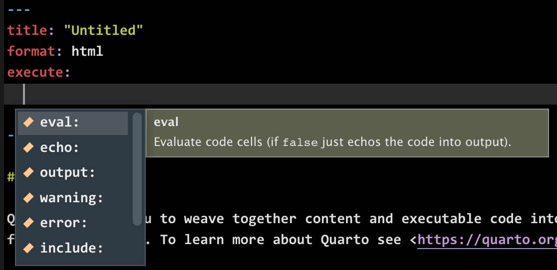
• Check HTML Options for more options!

```{r}
#| label: setup
#| include: false
# don't show code unless we explicitly set echo = TRUE
knitr::opts_chunk$set(echo = FALSE)
```

• knitr::opts_chunk$set() sets default options for all chunks.

Images

Basic markdown syntax:

![Maru](images/05-quarto/maru1.jpg)

Maru

Figures w/ code

```{r}
#| out-width: 40%
#| fig-align: right

knitr::include_graphics("images/05-quarto/maru1.jpg")
```

Width of the plot in the output document, which can be different from its physical fig-width, i.e., plots can be scaled in the output document. When used without a unit, the unit is assumed to be pixels. However, any of the following unit identifiers can be used: px, cm, mm, in, inch and %, for example, 3in, 8cm, 300px or 50%.

Including Plots

• Many chunk options for figures and images start with fig-, for example fig-width, fig-height, fig-show, etc.

```{r}
#| eval: false
#| fig-cap: "Fig. 1: Car stuff"
plot(x = cars$speed, y = cars$dist)
```

Fig. 1: Car stuff

Divs and Spans

This is text with [special]{style="color:red"} formatting.

This is text with special formatting.

::: {style="color:red"}
This content can be styled with a border
:::

This content can be styled with a border

Divs and Spans

• Think of a ::: div as a HTML <div> but it can also apply in specific situations to content in PDF

• [text]{.class} spans can be thought of a <span .class>Text</span>

  ::: {.border}
  This content can be styled with a border
  :::
  
  <div class="border">
    <p>This content can be styled with a border</p>
  </div>

<!-- ::: {style="border-left:10px solid red"} -->
<!-- This content can be styled with a border -->
<!-- ::: -->

Divs start with a fence containing at least three consecutive colons plus some attributes. The attributes may optionally be followed by another string of consecutive colons. The Div ends with another line containing a string of at least three consecutive colons. The Div should be separated by blank lines from preceding and following blocks.

Subfigures Fenced div Class

::: {#fig-maru layout-ncol=2}

![Loaf](images/05-quarto/maru2.jpg){#fig-loaf width="250px"}
![Lick](images/05-quarto/maru3.jpg){#fig-lick width="250px"}
Two states of Maru

:::

(a) Loaf

(b) Lick

Figure 1: Two states of Maru

Inline Code

• Inside your text you can include code with the syntax `r your-r-code`.
• For example, `r 4 + 5` would output 9 in your text.

head(cars)

  speed dist
1     4    2
2     4   10
3     7    4
4     7   22
5     8   16
6     9   10

num_cars <- nrow(cars)

Code in Quarto

There are `r num_cars` rows in the cars dataset. Four plus five is `r 4 + 5`

Output

There are 50 rows in the cars dataset. Four plus five is 9

• We;ve learned that Inside your text you can include code, and inline code is created with backticks.
• In fact, the inline code can actually execute code, if we put r in the first place.
• For example, 9 would output 9 in your text.

04-Code Chunk

• In lab.qmd ## Lab 4: Code Chunk, use code chunks to

  • include an image with knitr::include_graphics("URL or file path") https://raw.githubusercontent.com/rstudio/hex-stickers/master/PNG/ggplot2.png

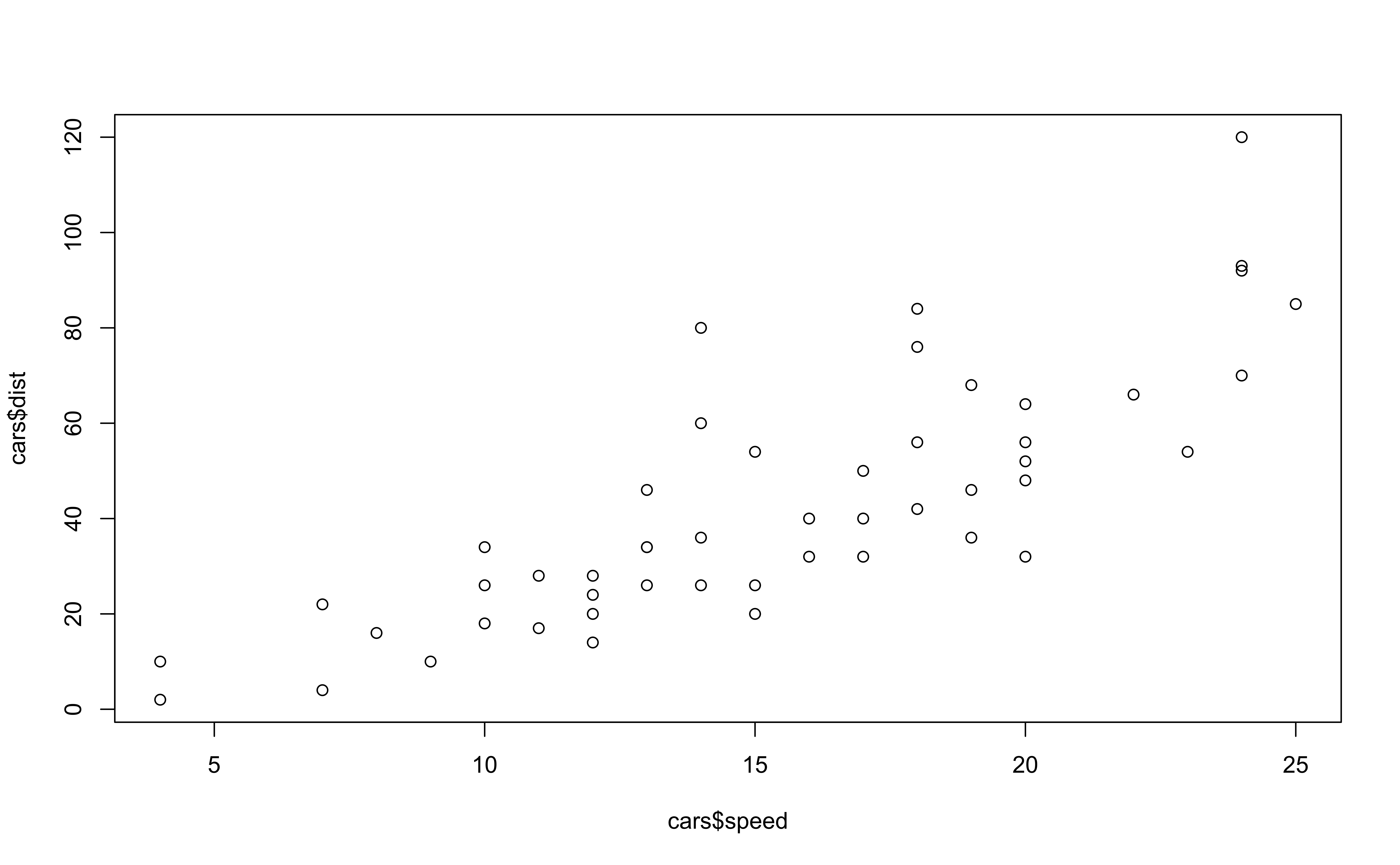
  • include a plot plot(mtcars$disp, mtcars$mpg)

  • Show dataset mtcars as a table using knitr::kable()

  • do some inline code calculation like `r ncol(mtcars)`, `r log(100, base = 10) + sqrt(4)`.

• Add option fig-height: 4, fig-width: 6 and fig-align: right to your plot. What are the changes?

• How do we set global chunk options to hide and run code in every chunk?

• Once done, commit with message “04-Code Chunk” and push your work to GitHub.

• Run the following in the console

Then, add the following chunk in your lab02-rmarkdown.qmd and re-knit it.

What happens? - The environment of your Quarto document is separate from the Console! Remember this, and expect it to bite you a few times as you’re learning to work with Quarto! - fig.dim = c(8, 6) means fig.width = 8 and fig.height = 6 in inches - out.width=“50%”: half of the width of the image container

Quarto Skills to the Next Level

• Quarto Website

• Get Started with Quarto

• R for Data Science Ch-28 Quarto