Basic R/Python

MATH/COSC 3570 Introduction to Data Science

Dr. Cheng-Han Yu
Department of Mathematical and Statistical Sciences
Marquette University

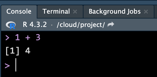
Run Code in Console

• reticulate::repl_python() to Python.

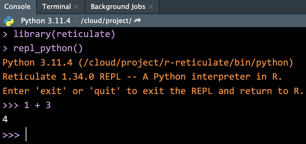
• quit or exit to change Console back to R.

Arithmetic and Logical Operators

2 + 3 / (5 * 4) ^ 2

[1] 2.01

5 == 5.00

[1] TRUE

# 5 and 5L are of the same value too
# 5 is of type double; 5L is integer
5 == 5L

[1] TRUE

typeof(5L)

[1] "integer"

!TRUE == FALSE

[1] TRUE

2 + 3 / (5 * 4) ** 2

2.0075

5 == 5.00

True

5 == int(5)

True

type(int(5))

<class 'int'>

not True == False

True

repl_python()

Arithmetic and Logical Operators

Type coercion: When doing AND/OR comparisons, all nonzero values are treated as TRUE and 0 as FALSE.

-5 | 0

[1] TRUE

1 & 1

[1] TRUE

2 | 0

[1] TRUE

bool() converts nonzero numbers to True and zero to False

-5 | 0

-5

1 & 1

1

bool(2) | bool(0)

True

Math Functions

Math functions in R are built-in.

sqrt(144)

[1] 12

exp(1)

[1] 2.72

sin(pi/2)

[1] 1

log(32, base = 2)

[1] 5

abs(-7)

[1] 7

# R comment

Need to import math library in Python.

import math
math.sqrt(144)

12.0

math.exp(1)

2.718281828459045

math.sin(math.pi/2)

1.0

math.log(32, 2)

5.0

abs(-7)

7

# python comment

Variables and Assignment

Use <- to do assignment. Why

## we create an object, value 5, 
## and call it x, which is a variable
x <- 5
x

[1] 5

(x <- x + 6)

[1] 11

x == 5

[1] FALSE

log(x)

[1] 2.4

Use = to do assignment.

x = 5
x

5

x = x + 6
x

11

x == 5

False

math.log(x)

2.3978952727983707

Object Types

character, double, integer and logical.

typeof(5)

[1] "double"

typeof(5L)

[1] "integer"

typeof("I_love_data_science!")

[1] "character"

typeof(1 > 3)

[1] "logical"

is.double(5L)

[1] FALSE

str, float, int and bool.

type(5.0)

<class 'float'>

type(5)

<class 'int'>

type("I_love_data_science!")

<class 'str'>

type(1 > 3)

<class 'bool'>

type(5) is float

False

python long (long integers, they can also be represented in octal and hexadecimal)

R Data Structures

• Vector

• Factor

• List

• Matrix

• Data Frame

• Variable defined previously is a scalar value, or in fact a (atomic) vector of length one.

(Atomic) Vector

• To create a vector, use c(), short for concatenate or combine.
• All elements of a vector must be of the same type.

(dbl_vec <- c(1, 2.5, 4.5)) 

[1] 1.0 2.5 4.5

(int_vec <- c(1L, 6L, 10L))

[1]  1  6 10

## TRUE and FALSE can be written as T and F
(log_vec <- c(TRUE, FALSE, F))  

[1]  TRUE FALSE FALSE

(chr_vec <- c("pretty", "girl"))

[1] "pretty" "girl"  

## check how many elements in a vector
length(dbl_vec) 

[1] 3

## check a compact description of 
## any R data structure
str(dbl_vec) 

 num [1:3] 1 2.5 4.5

Sequence of Numbers

• Use : to create a sequence of integers.
• Use seq() to create a sequence of numbers of type double with more options.

(vec <- 1:5) 

[1] 1 2 3 4 5

typeof(vec)

[1] "integer"

# a sequence of numbers from 1 to 10 with increment 2
(seq_vec <- seq(from = 1, to = 10, by = 2))

[1] 1 3 5 7 9

typeof(seq_vec)

[1] "double"

Operations on Vectors

• We can do any operations on vectors as we do on a scalar variable (vector of length 1).

# Create two vectors
v1 <- c(3, 8)
v2 <- c(4, 100) 

## All operations happen element-wisely
# Vector addition
v1 + v2

[1]   7 108

# Vector subtraction
v1 - v2

[1]  -1 -92

# Vector multiplication
v1 * v2

[1]  12 800

# Vector division
v1 / v2

[1] 0.75 0.08

sqrt(v2)

[1]  2 10

Recycling of Vectors

• If we apply arithmetic operations to two vectors of unequal length, the elements of the shorter vector will be recycled to complete the operations.

v1 <- c(3, 8, 4, 5)
# The following 2 operations are the same
v1 * 2

[1]  6 16  8 10

v1 * c(2, 2, 2, 2)

[1]  6 16  8 10

v3 <- c(4, 11)
v1 + v3  ## v3 becomes c(4, 11, 4, 11) when doing the operation

[1]  7 19  8 16

Subsetting Vectors

• To extract element(s) in a vector, we use a pair of brackets [] with element indexing.
• The indexing starts with 1.

v1

[1] 3 8 4 5

v2

[1]   4 100

## The 3rd element
v1[3] 

[1] 4

v1[c(1, 3)]

[1] 3 4

v1[1:2]

[1] 3 8

## extract all except a few elements
## put a negative sign before the vector of 
## indices
v1[-c(2, 3)] 

[1] 3 5

Factor

• A vector of type factor can be ordered in a meaningful way.
• Create a factor by factor(). It is a type of integer, not character. 😲 🙄

## Create a factor from a character vector using function factor()
(fac <- factor(c("med", "high", "low")))

[1] med  high low 
Levels: high low med

typeof(fac)  ## The type is integer.

[1] "integer"

str(fac)  ## The integers show the level each element in vector fac belongs to.

 Factor w/ 3 levels "high","low","med": 3 1 2

order_fac <- factor(c("med", "high", "low"),
                    levels = c("low", "med", "high"))
str(order_fac)

 Factor w/ 3 levels "low","med","high": 2 3 1

levels(fac) ## Each level represents an integer, ordered from the vector alphabetically.

List (Generic Vectors)

• Lists are different from (atomic) vectors: Elements can be of any type, including lists.

• Construct a list by using list().

## a list of 3 elements of different types
x_lst <- list(idx = 1:3, 
              "a", 
              c(TRUE, FALSE))

$idx
[1] 1 2 3

[[2]]
[1] "a"

[[3]]
[1]  TRUE FALSE

str(x_lst)

List of 3
 $ idx: int [1:3] 1 2 3
 $    : chr "a"
 $    : logi [1:2] TRUE FALSE

names(x_lst)

[1] "idx" ""    ""   

length(x_lst)

[1] 3

Subsetting a List

Return an element of a list

## subset by name (a vector)
x_lst$idx  

[1] 1 2 3

## subset by indexing (a vector)
x_lst[[1]]  

[1] 1 2 3

typeof(x_lst$idx)

[1] "integer"

Return a sub-list of a list

## subset by name (still a list)
x_lst["idx"]  

$idx
[1] 1 2 3

## subset by indexing (still a list)
x_lst[1]  

$idx
[1] 1 2 3

typeof(x_lst["idx"])

[1] "list"

• This is where we should pay more attention to. When we subset a list, it may return an element of the list, or it returns a sub-list of the list.
• Let’s see how it happens.
• This is our x_lst. We can subset a list by name or by indexing.
• Suppose we want the first element of the list, we can get it by its name using x_lst$idx.
• We can also obtain it by using indexing like x_lst[[1]] because we want the first element.
• Notice that the way we subset a list returns an integer vector, the real first element of the list, not a list.
• Let’s see another case on the right.
• We can also subset by name using single pair of brackets, and put the name inside the brackets.
• Or we can subset by indexing, again using single pair of brackets.
• And you see what happened? The way we subset a list here returns a sub-list, not the element itself.
• So please be careful when subsetting a list.
• If you want a vector, use these ways. If you want to keep it as a list, use these ways.

pepper packet pepper shaker

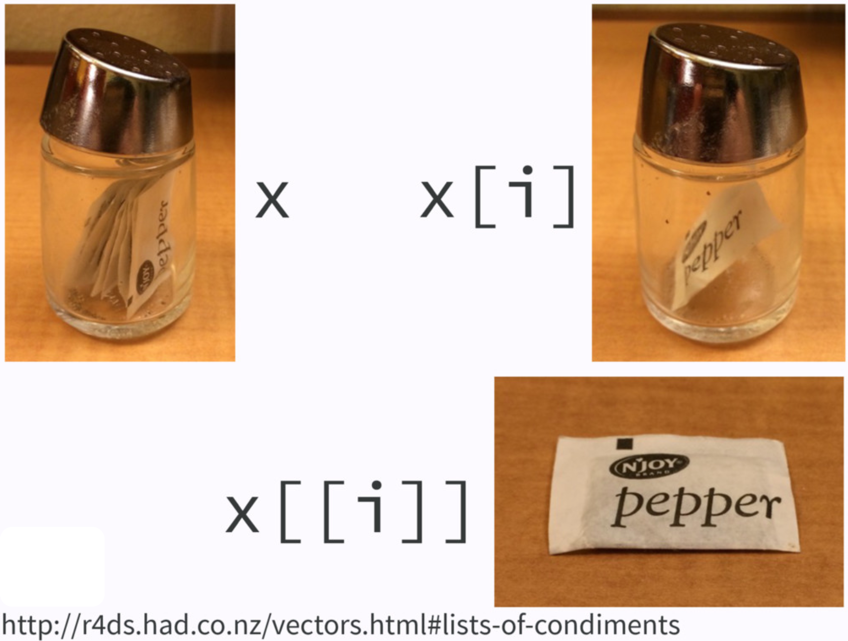
If list x is a train carrying objects, then x[[5]] is the object in car 5; x[4:6] is a train of cars 4-6.

— @RLangTip, https://twitter.com/RLangTip/status/268375867468681216

Matrix

• A matrix is a two-dimensional analog of a vector with attribute dim.
• Use command matrix() to create a matrix.

## Create a 3 by 2 matrix called mat
(mat <- matrix(data = 1:6, nrow = 3, ncol = 2)) 

     [,1] [,2]
[1,]    1    4
[2,]    2    5
[3,]    3    6

dim(mat); nrow(mat); ncol(mat)

[1] 3 2

[1] 3

[1] 2

     [,1] [,2]
[1,]    1    2
[2,]    3    4
[3,]    5    6

$dim
[1] 3 2

Row and Column Names

mat

     [,1] [,2]
[1,]    1    4
[2,]    2    5
[3,]    3    6

## assign row names and column names
rownames(mat) <- c("A", "B", "C")
colnames(mat) <- c("a", "b")
mat

  a b
A 1 4
B 2 5
C 3 6

rownames(mat)

[1] "A" "B" "C"

colnames(mat)

[1] "a" "b"

attributes(mat)

$dim
[1] 3 2

$dimnames
$dimnames[[1]]
[1] "A" "B" "C"

$dimnames[[2]]
[1] "a" "b"

Subsetting a Matrix

• Use the same indexing approach as vectors on rows and columns.
• Use comma , to separate row and column index.
• mat[2, 2] extracts the element of the second row and second column.

mat

  a b
A 1 4
B 2 5
C 3 6

## all rows and 2nd column
## leave row index blank
## specify 2 in coln index
mat[, 2]

A B C 
4 5 6 

## 2nd row and all columns
mat[2, ] 

a b 
2 5 

## The 1st and 3rd rows and the 1st column
mat[c(1, 3), 1] 

A C 
1 3 

Binding Matrices

• cbind() (binding matrices by adding columns)

• rbind() (binding matrices by adding rows)

• When matrices are combined by columns (rows), they should have the same number of rows (columns).

mat

  a b
A 1 4
B 2 5
C 3 6

mat_c <- matrix(data = c(7,0,0,8,2,6), 
                nrow = 3, ncol = 2)
## should have the same number of rows
cbind(mat, mat_c)  

  a b    
A 1 4 7 8
B 2 5 0 2
C 3 6 0 6

mat_r <- matrix(data = 1:4, 
                nrow = 2, 
                ncol = 2)
## should have the same number of columns
rbind(mat, mat_r)  

  a b
A 1 4
B 2 5
C 3 6
  1 3
  2 4

Data Frame: The Most Common Way of Storing Datasets

• A data frame is of type list of equal-length vectors, having a 2-dimensional structure.
• More general than matrix: Different columns can have different types.
• Use data.frame() that takes named vectors as input “element”.

## data frame w/ an dbl column named age
## and char column named gender.
(df <- data.frame(age = c(19, 21, 40), 
                  gen = c("m","f", "m")))

  age gen
1  19   m
2  21   f
3  40   m

## a data frame has a list structure
str(df)  

'data.frame':   3 obs. of  2 variables:
 $ age: num  19 21 40
 $ gen: chr  "m" "f" "m"

## must set column names
## or they are ugly and non-recognizable
data.frame(c(19,21,40), c("m","f","m")) 

  c.19..21..40. c..m....f....m..
1            19                m
2            21                f
3            40                m

Properties of Data Frames

Data frame has properties of matrix and list.

names(df)  ## df as a list

[1] "age" "gen"

colnames(df)  ## df as a matrix

[1] "age" "gen"

length(df) ## df as a list

[1] 2

ncol(df) ## df as a matrix

[1] 2

dim(df) ## df as a matrix

[1] 3 2

## rbind() and cbind() can be used on df
df_r <- data.frame(age = 10, 
                   gen = "f")
rbind(df, df_r)

  age gen
1  19   m
2  21   f
3  40   m
4  10   f

df_c <- 
    data.frame(col = c("red","blue","gray"))
(df_new <- cbind(df, df_c))

  age gen  col
1  19   m  red
2  21   f blue
3  40   m gray

Subsetting a Data Frame

Can use either list or matrix subsetting methods.

df_new

  age gen  col
1  19   m  red
2  21   f blue
3  40   m gray

## Subset rows
df_new[c(1, 3), ]

  age gen  col
1  19   m  red
3  40   m gray

## select the row where age == 21
df_new[df_new$age == 21, ]

  age gen  col
2  21   f blue

## Subset columns
## like a list
df_new$age

[1] 19 21 40

df_new[c("age", "gen")]

  age gen
1  19   m
2  21   f
3  40   m

## like a matrix
df_new[, c("age", "gen")]

  age gen
1  19   m
2  21   f
3  40   m

  age gen  col
1  19   m  red
3  40   m gray

'data.frame':   3 obs. of  1 variable:
 $ age: num  19 21 40

 num [1:3] 19 21 40

05-R Data Type Summary

In lab.qmd Lab 5,

• Create R objects vector v1, factor f2, list l3, matrix m4 and data frame d5.

• Check typeof() and class() of those objects, and create a list having the output below.

v1 <- __________
f2 <- __________
l3 <- __________
m4 <- __________
d5 <- __________
v <- c(type = typeof(v1), class = class(v1))
f <- c(type = __________, class = _________)
l <- c(type = __________, class = _________)
m <- c(type = __________, class = _________)
d <- c(type = __________, class = _________)
____(vec    =   v,
     ______ = ___,
     ______ = ___,
     ______ = ___,
     ______ = ___)

$vec
     type     class 
 "double" "numeric" 

$fac
     type     class 
"integer"  "factor" 

$lst
  type  class 
"list" "list" 

$mat
     type    class1    class2 
"integer"  "matrix"   "array" 

$df
        type        class 
      "list" "data.frame" 

Python Data Structures

• List

• Tuple

• Dictionary

Python Lists

• Python has numbers and strings, but no built-in vector structure.
• To create a sequence type of structure, we can use a list that can save several elements in an single object.
• To create a list in Python, we use [].

lst_num = [0, 2, 4] 
lst_num

[0, 2, 4]

type(lst_num)

<class 'list'>

len(lst_num)

3

List elements can have different types!

lst = ['data', 'math', 34, True]
lst

['data', 'math', 34, True]

Subsetting Lists

• Indexing in Python always starts at 0!
• 0: the 1st element

lst

['data', 'math', 34, True]

lst[0]

'data'

type(lst[0]) ## not a list

<class 'str'>

• -1: the last element

lst[-2]

34

• [a:b]: the (a+1)-th to b-th elements

lst[1:4]

['math', 34, True]

type(lst[1:4]) ## a list

<class 'list'>

• [a:]: elements from the (a+1)-th to the last

lst[2:]

[34, True]

What does lst[0:1] return? Is it a list?

What does lst[0:1] return? Is it a list?

Lists are Mutable

Lists are changed in place!

lst[1]

'math'

lst[1] = "stats"
lst

['data', 'stats', 34, True]

lst[2:] = [False, 77]
lst

['data', 'stats', False, 77]

If we change any element value in a list, the list itself will be changed as well.

List Operations and Methods list.method()

## Concatenation
lst_num + lst

[0, 2, 4, 'data', 'stats', False, 77]

## Repetition
lst_num * 3 

[0, 2, 4, 0, 2, 4, 0, 2, 4]

## Membership
34 in lst

False

## Appends "cat" to lst
lst.append("cat")
lst

['data', 'stats', False, 77, 'cat']

## Removes and returns last object from list
lst.pop()

'cat'

lst

['data', 'stats', False, 77]

## Removes object from list
lst.remove("stats")
lst

['data', False, 77]

## Reverses objects of list in place
lst.reverse()
lst

[77, False, 'data']

This is a common syntax in Python. We start with a Pyhton object of some type, then type dot followed by any method specifically for this particular data type or structure for operations. list.pop(index)

Tuples

• Tuples work exactly like lists except they are immutable, i.e., they can’t be changed in place.

• To create a tuple, we use ().

tup = ('data', 'math', 34, True)
tup

('data', 'math', 34, True)

type(tup)

<class 'tuple'>

len(tup)

4

tup[2:]

(34, True)

tup[-2]

34

tup[1] = "stats"  ## does not work!
# TypeError: 'tuple' object does not support item assignment

tup

('data', 'math', 34, True)

‘tuple’ object does not support item assignment

Tuples Functions and Methods

# Converts a list into tuple
tuple(lst_num)

(0, 2, 4)

# number of occurance of "data"
tup.count("data")

1

# first index of "data"
tup.index("data")

0

Note

Lists have more methods than tuples because lists are more flexible.

Dictionaries

• A dictionary consists of key-value pairs.

• A dictionary is mutable, i.e., the values can be changed in place and more key-value pairs can be added.

• To create a dictionary, we use {"key name": value}.

• The value can be accessed by the key in the dictionary.

dic = {'Name': 'Ivy', 'Age': 7, 'Class': 'First'}

dic['Age']

7

dic['age']  ## does not work

dic['Age'] = 9
dic['Class'] = 'Third'
dic

{'Name': 'Ivy', 'Age': 9, 'Class': 'Third'}

Properties of Dictionaries

• Python will use the last assignment!

dic1 = {'Name': 'Ivy', 'Age': 7, 'Name': 'Liya'}
dic1['Name']

'Liya'

• Keys are unique and immutable.

• A key can be a tuple, but CANNOT be a list.

## The first key is a tuple!
dic2 = {('First', 'Last'): 'Ivy Lee', 'Age': 7}
dic2[('First', 'Last')]

'Ivy Lee'

## does not work
dic2 = {['First', 'Last']: 'Ivy Lee', 'Age': 7}
dic2[['First', 'Last']]

Disctionary Methods

{'Name': 'Ivy', 'Age': 9, 'Class': 'Third'}

## Returns list of dictionary dict's keys
dic.keys()

dict_keys(['Name', 'Age', 'Class'])

## Returns list of dictionary dict's values
dic.values()

dict_values(['Ivy', 9, 'Third'])

## Returns a list of dict's (key, value) tuple pairs
dic.items()

dict_items([('Name', 'Ivy'), ('Age', 9), ('Class', 'Third')])

## Adds dictionary dic2's key-values pairs in to dic
dic2 = {'Gender': 'female'}
dic.update(dic2)
dic

{'Name': 'Ivy', 'Age': 9, 'Class': 'Third', 'Gender': 'female'}

## Removes all elements of dictionary dict
dic.clear()
dic

{}

06-Python Data Structure

In lab.qmd Lab 6,

• Create a Python list and dictionary similar to the R list below.

x_lst <- list(idx = 1:3, 
              "a", 
              c(TRUE, FALSE))

Remember to create Python code chunk

```{Python}
#| echo: true
#| eval: false

```

Any issue of this Python chunk?

Commit and Push your work once you are done.

Python Data Structures for Data Science

• Python built-in data structures are not specifically for data science.

• To use more data science friendly functions and structures, such as array or data frame, Python relies on packages NumPy and pandas.

Installing NumPy and pandas*

In your lab-yourusername project, run

library(reticulate)
virtualenv_create("myenv")

Go to Tools > Global Options > Python > Select > Virtual Environments

Installing NumPy and pandas*

You may need to restart R session. Do it, and in the new R session, run

library(reticulate)
py_install(c("numpy", "pandas", "matplotlib"))

Run the following Python code, and make sure everything goes well.

import numpy as np
import pandas as pd
v1 = np.array([3, 8])
v1
df = pd.DataFrame({"col": ['red', 'blue', 'green']})
df

Descriptive Statistics (MATH 4720)

• Central Tendency and Variability

• Data Summary

Central Tendency: Mean and Median

data <- c(3,12,56,9,230,22)
mean(data)

[1] 55.3

median(data)  

[1] 17

data = np.array([3,12,56,9,230,22])
type(data)

<class 'numpy.ndarray'>

np.mean(data)

55.333333333333336

np.median(data)

17.0

• The (arithmetic) mean or average is adding up all of the values, then dividing by the total number of them.
• Mean balances data Values.
• The median is the middle value when data values are arranged from the lowest to highest.
• Mean is sensitive to extreme values (outliers).

Variation

quantile(data, c(0.25, 0.5, 0.75)) 

  25%   50%   75% 
 9.75 17.00 47.50 

var(data)

[1] 7677

sd(data)

[1] 87.6

summary(data)

   Min. 1st Qu.  Median    Mean 3rd Qu.    Max. 
    3.0     9.8    17.0    55.3    47.5   230.0 

np.quantile(data,  [0.25, 0.5, 0.75])

array([ 9.75, 17.  , 47.5 ])

np.var(data, ddof = 1)

7676.666666666666

np.std(data, ddof = 1)

87.61658899242008

df = pd.Series(data)
df.describe()

count      6.000000
mean      55.333333
std       87.616589
min        3.000000
25%        9.750000
50%       17.000000
75%       47.500000
max      230.000000
dtype: float64

• p-th percentile: a data value such that at most \(p\%\) of the data values are below it and at most \((1−p)\%\) of the values are above it.
• First Quartile (Q1): the 25-th percentile
• Second Quartile (Q2): the 50-th percentile (Median)
• Third Quartile (Q3): the 75-th percentile
• Interquartile Range (IQR): Q3 - Q1 IQR(data)

q75, q25 = np.percentile(data, [75 ,25])
q75 - q25

37.75

Delta Degrees of Freedom.

Basic Plotting

• Scatter Plot

• Boxplot

• Histogram

• Bar Chart

• Pie Chart

• 2D Imaging

• 3D Plotting

R plot()

mtcars[1:15, 1:4]

                    mpg cyl disp  hp
Mazda RX4          21.0   6  160 110
Mazda RX4 Wag      21.0   6  160 110
Datsun 710         22.8   4  108  93
Hornet 4 Drive     21.4   6  258 110
Hornet Sportabout  18.7   8  360 175
Valiant            18.1   6  225 105
Duster 360         14.3   8  360 245
Merc 240D          24.4   4  147  62
Merc 230           22.8   4  141  95
Merc 280           19.2   6  168 123
Merc 280C          17.8   6  168 123
Merc 450SE         16.4   8  276 180
Merc 450SL         17.3   8  276 180
Merc 450SLC        15.2   8  276 180
Cadillac Fleetwood 10.4   8  472 205

plot(x = mtcars$mpg, y = mtcars$hp, 
     xlab  = "Miles per gallon", 
     ylab = "Horsepower", 
     main = "Scatter plot", 
     col = "red", 
     pch = 5, las = 1)

Argument pch

• The defualt is pch = 1

Python matplotlib.pyplot

mtcars = pd.read_csv('./data/mtcars.csv')
mtcars.iloc[0:15,0:4]

     mpg  cyl   disp   hp
0   21.0    6  160.0  110
1   21.0    6  160.0  110
2   22.8    4  108.0   93
3   21.4    6  258.0  110
4   18.7    8  360.0  175
5   18.1    6  225.0  105
6   14.3    8  360.0  245
7   24.4    4  146.7   62
8   22.8    4  140.8   95
9   19.2    6  167.6  123
10  17.8    6  167.6  123
11  16.4    8  275.8  180
12  17.3    8  275.8  180
13  15.2    8  275.8  180
14  10.4    8  472.0  205

import matplotlib.pyplot as plt
plt.scatter(x = mtcars.mpg, 
            y = mtcars.hp, 
            color = "r")
plt.xlabel("Miles per gallon")
plt.ylabel("Horsepower")
plt.title("Scatter plot")

Python Subplots

Note

The command plt.scatter() is used for creating one single plot. If multiple subplots are wanted in one single call, one can use the format

fig, (ax1, ax2) = plt.subplots(1, 2)
ax1.scatter(x, y)
ax2.plot(x, y)

• Check Creating multiple subplots using plt.subplots for more details.

R Subplots

par(mfrow = c(1, 2))
plot(x = mtcars$mpg, y = mtcars$hp, xlab = "mpg")
plot(x = mtcars$mpg, y = mtcars$weight, xlab = "mpg")

R boxplot()

boxplot(mpg ~ cyl, 
        data = mtcars, 
        col = c("blue", "green", "red"), 
        las = 1, 
        horizontal = TRUE,
        xlab = "Miles per gallon", 
        ylab = "Number of cylinders")

• Visualizing relationships between numerical and categorical data, we can check side-by-side boxplots.
• For example, if we want to check the data variation of (miles per gallon) for each number of cylinder, we can use boxplot() function.
• And inside the function, we use the formula mpg ~ cyl, and specify the dataset.
• That is basically it. The rest of arguments are decorating your plot. They are optional.

Python boxplot()

cyl_index = np.sort(np.unique(np.array(mtcars.cyl)))
cyl_shape = cyl_index.shape[0]
cyl_list = []
for i in range (0, cyl_shape):
    cyl_list.append(np.array(mtcars[mtcars.cyl == cyl_index[i]].mpg))

import matplotlib.pyplot as plt
plt.boxplot(cyl_list, vert=False, labels=[4, 6, 8])

plt.xlabel("Miles per gallon")
plt.ylabel("Number of cylinders")

R hist()

• hist() decides the class intervals/with based on breaks. If not provided, R chooses one.

hist(mtcars$wt, 
     breaks = 20, 
     col = "#003366", 
     border = "#FFCC00", 
     xlab = "weights", 
     main = "Histogram of weights",
     las = 1)

• Besides color names, you can also use hex number to specify colors. Pretty handy.

Python hist()

plt.hist(mtcars.wt, 
         bins = 19, 
         color="#003366",
         edgecolor="#FFCC00")
plt.xlabel("weights")
plt.title("Histogram of weights")

R barplot()

(counts <- table(mtcars$gear)) 

 3  4  5 
15 12  5 

my_bar <- barplot(counts, 
                  main = "Car Distribution", 
                  xlab = "Number of Gears", 
                  las = 1)
text(x = my_bar, y = counts - 0.8, 
     labels = counts, 
     cex = 0.8)

Python barplot()

count_py = mtcars.value_counts('gear')
count_py

gear
3    15
4    12
5     5
Name: count, dtype: int64

plt.bar(count_py.index, count_py)
plt.xlabel("Number of Gears")
plt.title("Car Distribution")

R pie()

(percent <- round(counts / sum(counts) * 100, 2))

   3    4    5 
46.9 37.5 15.6 

(labels <- paste0(3:5, " gears: ", percent, "%"))

[1] "3 gears: 46.88%" "4 gears: 37.5%"  "5 gears: 15.62%"

pie(x = counts, labels = labels,
    main = "Pie Chart", 
    col = 2:4, 
    radius = 1)

• Pie charts are used for categorical variables, especially when we want to know percentage of each category.
• The first argument is the frequency table, and you can add labels to each category.

Python pie()

percent = round(count_py / sum(count_py) * 100, 2)
texts = [str(percent.index[k]) + " gear " + str(percent.array[k]) + "%" for k in range(0,3)]

plt.pie(count_py, labels = texts, colors = ['r', 'g', 'b'])

plt.title("Pie Charts")

R 2D Imaging: image()

• The image() function displays the values in a matrix using color.

matrix(1:30, 6, 5)

     [,1] [,2] [,3] [,4] [,5]
[1,]    1    7   13   19   25
[2,]    2    8   14   20   26
[3,]    3    9   15   21   27
[4,]    4   10   16   22   28
[5,]    5   11   17   23   29
[6,]    6   12   18   24   30

image(matrix(1:30, 6, 5))

In Python,

plt.imshow(mat_img, cmap='Oranges')

R fields::image.plot()

library(fields)
str(volcano)

 num [1:87, 1:61] 100 101 102 103 104 105 105 106 107 108 ...

image.plot(volcano)

R 2D Imaging Example: Volcano

R 3D scatter plot: scatterplot3d()

library("scatterplot3d")
scatterplot3d(x = mtcars$wt, 
              y = mtcars$disp, 
              z = mtcars$mpg, 
              main = "3D Scatter Plot", 
              xlab = "Weights", 
              ylab = "Displacement",
              zlab = "Miles per gallon", 
              pch = 16, 
              color = "steelblue")

In Python,

fig = plt.figure()
ax = fig.add_subplot(projection='3d')

R Perspective Plot: persp()

# Exaggerate the relief
z <- 2 * volcano      
# 10 meter spacing (S to N)
x <- 10 * (1:nrow(z))   
# 10 meter spacing (E to W)
y <- 10 * (1:ncol(z))   
par(bg = "slategray")
persp(x, y, z, 
      theta = 135, 
      phi = 30, 
      col = "green3", 
      scale = FALSE,
      ltheta = -120, 
      shade = 0.75, 
      border = NA, 
      box = FALSE)

In Python,

fig, ax = plt.subplots(subplot_kw={"projection": "3d"})
ax.plot_surface(X, Y, Z)

• You can also generate a so-called perspective plot using the function persp().
• I don’t use the function often. You can try it with different argument values, and see how it changes.

07-Plotting (Bonus question!)

In lab.qmd ## Lab 7,

• For the mtcars data, use R or Python to

  • make a scatter plot of miles per gallon vs. weight. Decorate your plot using arguments, col, pch, xlab, etc.

  • create a histogram of 1/4 mile time. Make it beautiful!

• Commit and Push your work once you are done.

import pandas as pd
import matplotlib.pyplot as plt
mtcars = pd.read_csv('./data/mtcars.csv')

• Find your mate and work in pairs.

• Two volunteer pairs teach us how to make beautiful plots next Tuesday (Feb 13)!

• The presenters will be awarded a hex sticker! 😎

Resources

• The R Graph Gallery
• matplotlib

We will talk about data visualization in detail soon!

https://stackoverflow.com/questions/43482191/matplotlib-axes-plot-vs-pyplot-plot