Data Importing

MATH/COSC 3570 Introduction to Data Science

Dr. Cheng-Han Yu
Department of Mathematical and Statistical Sciences
Marquette University

DBI, jsonline, xml2, httr

R Data Importing

• There are tons of packages and tools out there, and there are lots of data file formats too.
• Due to time limit, we will just cover commonly used tools and data file formats. And I think that should be enough for you to do your own project.
• If you really need to import a data set that is stored in a very weird format, let me know. And we’ll see how to solve this problem, maybe transform the format into another format. OK.
• Here are the packages related to reading and writing files. We’ll talk about some of them today.

Rectangular Data

readr 📦 Functions

Function	Format	Typical suffix
read_table()	white space separated values	txt
read_csv()	comma separated values	csv
read_csv2()	semicolon separated values	csv
read_tsv()	tab delimited separated values	tsv
read_fwf()	fixed width files	txt
read_delim()	general text file format, must define delimiter	txt

Be careful: The suffix usually tells us what type of file it is, but no guarantee that these always match.

readr::read_lines("./data/murders.csv", n_max = 3)  ## there is a header

[1] "state,abb,region,population,total" "Alabama,AL,South,4779736,135"     
[3] "Alaska,AK,West,710231,19"         

• readr provides the following functions to read your data into R.
• Be careful: The suffix usually tells us what type of file it is, but no guarantee that these always match.
• If you don’t want to open your data file, you can read several lines of your data in R using the function read_lines().
• For example, I check the first three lines of the murders.csv file. And yes, it is a comma-separated-value or csv file.
• Fixed width text files are special cases of text files where the format is specified by column widths, pad character and left/right alignment. Column widths are measured in units of characters. For example, if you have data in a text file where the first column always has exactly 10 characters, and the second column has exactly 5, the third has exactly 12 (and so on), this would be categorized as a fixed width text file.

Reading Data

read_csv() prints out a column specification giving us delimiter, name and type of each column.

murders_csv <- read_csv(file = "./data/murders.csv")
# ── Column specification ─────────────
# Delimiter: ","
# chr (3): state, abb, region
# dbl (2): population, total
head(murders_csv)

# A tibble: 6 × 5
  state      abb   region population total
  <chr>      <chr> <chr>       <dbl> <dbl>
1 Alabama    AL    South     4779736   135
2 Alaska     AK    West       710231    19
3 Arizona    AZ    West      6392017   232
4 Arkansas   AR    South     2915918    93
5 California CA    West     37253956  1257
6 Colorado   CO    West      5029196    65

## View data in RStudio
view(murders_csv)

• OK. Let’s try to read the murders.csv file into R. We use read_csv(), and in the first argument, we tell R its file path. Your path is generally not the same as my path, so you get to change it to your path.
• When we run read_csv(), it prints out a column specification that gives the name and type of each column.
• You can see the data set is actually the one in the dslabs package, and we use it in a previous lab exercise, right?

Missing Values

Which type is the column vector x? Why?

• Type coercion¹ happens and all column elements are transformed to character type.

read_csv("./data/df-na.csv")

# A tibble: 9 × 3
  x     y              z     
  <chr> <chr>          <chr> 
1 1     a              hi    
2 <NA>  b              hello 
3 3     Not applicable 9999  
4 4     d              ola   
5 5     e              hola  
6 .     f              whatup
7 7     g              wassup
8 8     h              sup   
9 9     i              <NA>  

• I have a csv file with 3 columns x, y, and z.
• It looks like it should be some sort of numeric data. Right I have bunch of numbers here.
• Character string NA, but that’s just an NA. We have a period here, which is usually used as an NA as well.
• But when we read this into R, we can see that it’s being read as a character.
• The reason is that the period which is a character shows up, and type coercion happens and all column elements are transformed to character type.
• How to solve this kind of problem. We want x to be double and the period is actually a missing value.
• Imaging that if you have thousands of lines, you could very easily miss that period.

1. A column with elements having different types, they’ll be coerced to the most flexible type. Types from least to most flexible: logical – integer – double – character.

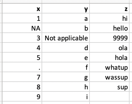
Solution 1: Explicit NAs

• By default, read_csv() only recognizes ” “ and NA as a missing value.
• Specify the values that are used to represent missing values by argument na.

read_csv("./data/df-na.csv", 
         na = c("", "NA", ".", "9999", "Not applicable"))

# A tibble: 9 × 3
      x y     z     
  <dbl> <chr> <chr> 
1     1 a     hi    
2    NA b     hello 
3     3 <NA>  <NA>  
4     4 d     ola   
5     5 e     hola  
6    NA f     whatup
7     7 g     wassup
8     8 h     sup   
9     9 i     <NA>  

• The function recognize string NA as missing value, but not period or any other character or strings.
• One solution is to specify explicitly the value (or values) that are used to represent missing values.
• If you know what sort of character are used to denote missing values in your data file, you can give those as part of na argument in the read_csv() function.
• For example here, I treat ““,”NA”, “.”, “9999”, “Not applicable” all as missing values.
• And now the class of x is double, and all those character strings are denoted as NA in the loaded data set.

Solution 2: Specify Column Types

read_csv("./data/df-na.csv", 
         col_types = 
             cols(col_double(), 
                  col_character(), 
                  col_character()))

# A tibble: 9 × 3
      x y              z     
  <dbl> <chr>          <chr> 
1     1 a              hi    
2    NA b              hello 
3     3 Not applicable 9999  
4     4 d              ola   
5     5 e              hola  
6    NA f              whatup
7     7 g              wassup
8     8 h              sup   
9     9 i              <NA>  

# Warning message:
# One or more parsing issues, 
# call `problems()` 
# on your data frame for details

problems()
# A tibble: 1 × 5
#     row   col expected actual file 
#   <int> <int> <chr>    <chr>  <chr>
# 1     7     1 a double .      "" 

• Another solution is to specify column types when you import your data.
• This might be handy when you know what your column types should be.
• For example, here I can specify the column types using the col_types argument.
• All column types are wrapped up in the cols() command, that x is double, y is character and z is character as well.
• Ans now you can see x becomes double.
• And here we actually get a warning. In row 6 and col x, we expect a double but it is actually a dot or period, which is a character, and so R treats it as NA, which is exactly what I want to do.
• But R send a message telling us about this, and make sure this is what we want to do.
• This option might be preferable if you cannot scan your data file, or don;t know what convention is being used for missing values in your data file, but you happen to know your column types.
• The downside of this is that, here, Not applicable and 9999, they are all treated as valid character values, and they are not missing values. So be careful about this. You may need to manually clean your data.

Column Types

type function	data type
col_character()	character
col_date()	date
col_datetime()	POSIXct (date-time)
col_double()	double (numeric)
col_factor()	factor
col_guess()	let readr guess (default)
col_integer()	integer
col_logical()	logical
col_number()	numbers mixed with non-number characters
col_numeric()	double or integer
col_skip()	do not read
col_time()	time

• Here shows all possible column types you can use when importing your data into R. No need to memorize it. But just aware of them, and use them when you need to.

Writing Data

## Create tibbles using a row-by-row layout
(df <- tribble(
  ~x, ~y,
  1,  "a",
  2,  "b",
  3,  "c"
))

# A tibble: 3 × 2
      x y    
  <dbl> <chr>
1     1 a    
2     2 b    
3     3 c    

## same as tibble(x = 1:3, y = c(a, b, c))

## save data to "./data/df.csv"
df |> write_csv(file = "./data/df.csv")

• We can also write our data to a csv file as well.
• Here I create a tibble called df, and then I use write_csv() function to write the data set df to the file df.csv.

read_rds() and write_rds()

• We save an R object (usually a data set) in .Rds in the R binary file format. ¹

readr::write_rds(cars, 
                 file = "./data/cars.rds") 
# fs::dir_ls(path = "./data") |> head(10) (Check Files using fs)

my_car <- readr::read_rds(file = "./data/cars.rds") 
head(my_car, 3)

  speed dist
1     4    2
2     4   10
3     7    4

• We save an R object (usually a data set) in .Rdsm the R binary file format.
• Remember we talked about RData format last time, right?
• R provides two file formats of its own for storing data, .RDS and .RData. RDS files can store a single R object, and RData files can store multiple R objects.
• Usually, if we save a data set, we use .Rds, and if we save several objects, and the objects are some variables or functions, we use .RData.
• Read the data back into R.

1. Check R built-in data sets using command data().

10-Import Data

• If you haven’t, install and load the tidyverse package.

In lab.qmd ## Lab 10 section,

• Import ssa_male_prob.csv and ssa_female_prob.Rds in the data folder using read_csv() and call them ssa_male and ssa_female, respectively.

ssa_male <- readr::read____(____________)
ssa_female <- readr::read____(____________)

• Plot Age (x-axis) vs. LifeExp (y-axis) for Female. The type should be “line”, and the line color is red. Add x-label, y-label and title to your plot.

plot(x = _____, y = _____, type = ______, col = ______,
     xlab = ______, ylab = _______, main = ____________)

• Use lines() to add a line of Age (x-axis) vs. LifeExp (y-axis) for Male to the plot. The color is blue.

lines(x = _____, y = _____, col = ______)

library(tidyverse)
ssa <- read_csv(file = "./data/ssa-death-probability.csv")
ssa_male <- ssa[ssa$Sex == "Male", ]
ssa_female <- ssa[ssa$Sex == "Female", ]
plot(x = ssa_female$Age, y = ssa_female$LifeExp, 
     type = "l", col = 2, lwd = 3,
     xlab = "Age", ylab = "Life Exp",
     main = "Age vs. Life Exp by Gender")
lines(ssa_male$Age, ssa_male$LifeExp, col = 4, lwd = 3)

Read Excel Data

• Last time, we use the readr package to import our data into R, right?
• What if you have a data set stored in microsoft excel, well we can use read excel package to read your data.

readxl 📦 Functions

Function	Format	Typical suffix
read_excel()	auto detect the format	xls, xlsx
read_xls()	original format	xls
read_xlsx()	new format	xlsx

• The Microsoft Excel can have more than one sheet in one file.
• The functions above read the first sheet by default.
• The excel_sheets() gives us the names of all the sheets in an Excel file.

library(readxl)
excel_sheets("./data/2010_bigfive_regents.xls")

[1] "Sheet1" "Sheet2" "Sheet3"

• Here shows the main read excel functions. They are pretty similar to readr functions, but this time, your data file is not a text file, but a microsoft excel file.
• The Microsoft Excel can have more than one sheet in one file.
• The functions listed above read the first sheet by default.
• If you don’t want open your excel file and check its sheet names, the excel_sheets() function gives us the names of all the sheets in an Excel file.

Sheet Names

• The sheet names can be passed to the sheet argument to read sheets other than the first.

excel_sheets("./data/2010_bigfive_regents.xls")

[1] "Sheet1" "Sheet2" "Sheet3"

(data_xls <- read_xls(path = "./data/2010_bigfive_regents.xls", 
                      sheet = "Sheet3", skip = 1))

# A tibble: 19 × 6
  Scores `131024` `113804` `104201` `103886` `91756`
   <dbl>    <dbl>    <dbl>    <dbl>    <dbl>   <dbl>
1     10       NA       64        8      227      34
2     11        6       83       11      217      58
3     12       23       87        7       28      67
4     13        1       54       16      230      42
5     14        3      145       18      303      57
6     15       58      151       50      192      98
7     16        1      129       13      156     125
8     17       73      214       59      163     115
# ℹ 11 more rows

• The sheet names can be passed to the sheet argument in the functions to read sheets other than the first.
• For example, here we ask R to read the Sheet1 in the favourite-food excel file.
• We can also specify an integer that indicates the position of the sheet.
• We don’t have a lab exercise on this. You have data and code is right here. You can practice and see if you can read the excel file.

pd.read_csv

pd.read_excel

pd.DataFrame.to_csv

pd.read_csv

import numpy as np
import pandas as pd

py_df = pd.read_csv('./data/murders.csv')
py_df.head()

        state abb region  population  total
0     Alabama  AL  South     4779736    135
1      Alaska  AK   West      710231     19
2     Arizona  AZ   West     6392017    232
3    Arkansas  AR  South     2915918     93
4  California  CA   West    37253956   1257

pd.DataFrame.to_csv

w = {"x":[1, 2, 3], 
     "y":['a', 'b','c']}
wdf = pd.DataFrame(w)

wdf.to_csv("./data/wdf.csv")
mydf = pd.read_csv('./data/wdf.csv')
mydf.head()

   Unnamed: 0  x  y
0           0  1  a
1           1  2  b
2           2  3  c

## index = False means don't write row names
wdf.to_csv("./data/wdf.csv", index = False)
mydf = pd.read_csv('./data/wdf.csv')
mydf.head()

   x  y
0  1  a
1  2  b
2  3  c