
Data Wrangling - one data frame 🛠
MATH/COSC 3570 Introduction to Data Science
Dr. Cheng-Han Yu
Department of Mathematical and Statistical Sciences
Marquette University
Department of Mathematical and Statistical Sciences
Marquette University
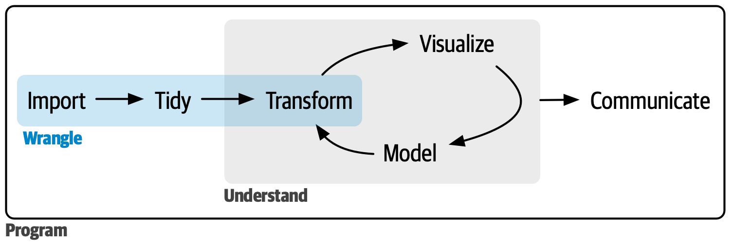
Grammar of Data Manipulation
Grammar of Data Wrangling: dplyr 📦
- based on the concepts of functions as verbs that manipulate data frames
-
mutate: create new columns from the existing1 -
filter: pick rows matching criteria -
slice: pick rows using index(es) -
distinct: filter for unique rows -
select: pick columns by name -
summarise: reduce variables to values -
group_by: for grouped operations -
arrange: reorder rows - … (many more)
Rules of dplyr Functions
First argument is always a data frame
Subsequent arguments say what to do with that data frame
Always return a data frame
Don’t modify in place
Data: US gun murders by state for 2010
# A tibble: 51 × 5
  state      abb   region population total
  <chr>      <chr> <chr>       <dbl> <dbl>
1 Alabama    AL    South     4779736   135
2 Alaska     AK    West       710231    19
3 Arizona    AZ    West      6392017   232
4 Arkansas   AR    South     2915918    93
5 California CA    West     37253956  1257
6 Colorado   CO    West      5029196    65
# ℹ 45 more rowsAdding a New Variable (Column) with mutate()
-
dplyr::mutate()takes- a data frame as the 1st argument
- the name and values of the variable as the 2nd argument using format
name = values.
# A tibble: 51 × 6
  state      abb   region population total  rate
  <chr>      <chr> <chr>       <dbl> <dbl> <dbl>
1 Alabama    AL    South     4779736   135  2.82
2 Alaska     AK    West       710231    19  2.68
3 Arizona    AZ    West      6392017   232  3.63
4 Arkansas   AR    South     2915918    93  3.19
5 California CA    West     37253956  1257  3.37
6 Colorado   CO    West      5029196    65  1.29
# ℹ 45 more rowstotalandpopulationinside the function are not defined in our R environment.dplyrfunctions know to look for variables in the data frame provided in the 1st argument.
Filtering Observations (Rows) with filter()
-
dplyr::filter()takes a- data frame as the 1st argument
- conditional statement as the 2nd. (pick rows matching criteria)
# filter the data table to only show the entries for which
# the murder rate is lower than 0.7
murders |>
    filter(rate < 0.7) #<<
# A tibble: 5 × 6
state abb region population total rate
<chr> <chr> <chr> <dbl> <dbl> <dbl>
1 Hawaii HI West 1360301 7 0.515
2 Iowa IA North Central 3046355 21 0.689
3 New Hampshire NH Northeast 1316470 5 0.380
4 North Dakota ND North Central 672591 4 0.595
5 Vermont VT Northeast 625741 2 0.320
filter() for Many Conditions at Once
Logical Operators
| operator | definition | operator | definition |
|---|---|---|---|
< |
less than |
x | y
|
x OR y
|
<= |
less than or equal to | is.na(x) |
if x is NA
|
> |
greater than | !is.na(x) |
if x is not NA
|
>= |
greater than or equal to | x %in% y |
if x is in y
|
== |
exactly equal to | !(x %in% y) |
if x is not in y
|
!= |
not equal to | !x |
not x
|
x & y |
x AND y
|
slice() for Certain Rows using Indexes
# A tibble: 4 × 6
  state      abb   region population total  rate
  <chr>      <chr> <chr>       <dbl> <dbl> <dbl>
1 Arizona    AZ    West      6392017   232  3.63
2 Arkansas   AR    South     2915918    93  3.19
3 California CA    West     37253956  1257  3.37
4 Colorado   CO    West      5029196    65  1.29
How do we subset rows using matrix indexing?
distinct() to Filter for Unique Rows
# A tibble: 4 × 1
  region
  <chr>
1 South
2 West
3 Northeast
4 North Central# A tibble: 4 × 6
state abb region population total rate
<chr> <chr> <chr> <dbl> <dbl> <dbl>
1 Alabama AL South 4779736 135 2.82
2 Alaska AK West 710231 19 2.68
3 Connecticut CT Northeast 3574097 97 2.71
4 Illinois IL North Central 12830632 364 2.84
distinct() Grabs First Row of The Unique Value
# A tibble: 4 × 6
  state       abb   region        population total  rate
  <chr>       <chr> <chr>              <dbl> <dbl> <dbl>
1 Alabama     AL    South            4779736   135  2.82
2 Alaska      AK    West              710231    19  2.68
3 Connecticut CT    Northeast        3574097    97  2.71
4 Illinois IL North Central 12830632 364 2.84Selecting Columns with select()
- In
dplyr::select(), the 1st argument is a data frame, followed by variable names being selected in the data. - The order of variable names matters!
select() to Exclude Variables
# A tibble: 51 × 5
state abb region total rate
<chr> <chr> <chr> <dbl> <dbl>
1 Alabama AL South 135 2.82
2 Alaska AK West 19 2.68
3 Arizona AZ West 232 3.63
4 Arkansas AR South 93 3.19
5 California CA West 1257 3.37
6 Colorado CO West 65 1.29
# ℹ 45 more rows
select() a Range of Variables
[1] "state"      "abb"        "region"     "population" "total"
[6] "rate"
# A tibble: 51 × 4
region population total rate
<chr> <dbl> <dbl> <dbl>
1 South 4779736 135 2.82
2 West 710231 19 2.68
3 West 6392017 232 3.63
4 South 2915918 93 3.19
5 West 37253956 1257 3.37
6 West 5029196 65 1.29
# ℹ 45 more rows
select() Variables with Certain Characteristics
-
starts_with()is a tidy-select helper function.
select() Variables with Certain Characteristics
-
ends_with()is a tidy-select helper function.
tidy-select Helpers1
-
starts_with(): Starts with a prefix -
ends_with(): Ends with a suffix -
contains(): Contains a literal string -
num_range(): Matches a numerical range like x01, x02, x03 -
one_of(): Matches variable names in a character vector -
everything(): Matches all variables -
last_col(): Select last variable, possibly with an offset -
matches(): Matches a regular expression (a sequence of symbols/characters expressing a string/pattern to be searched for within text)
Rationale for Pipe Operator
How do we show three variables (state, region, rate) for states that have murder rates below 0.7?
- Method 1: Define the intermediate object
new_table
Rationale for Pipe Operator
How do we show three variables (state, region, rate) for states that have murder rates below 0.7?
- Method 2: Apply one function onto the other with no intermediate object
Rationale for Pipe Operator
- The code that looks like a verbal description of what we want to do without intermediate objects:
data > select() > data after selecting > filter() > data after selecting and filtering
Summarizing Data – summarize()
-
summarize()provides a data frame that summarizes the statistics we compute.
Summarizing Data – summarize()
(s <- heights |>
    filter(sex == "Female") |>
    summarize(avg = mean(height),
              stdev = sd(height),
              median = median(height),
              minimum = min(height)))
# A tibble: 1 × 4
avg stdev median minimum
<dbl> <dbl> <dbl> <dbl>
1 64.9 3.76 65.0 51[1] 64.9[1] 51summarise() produces a new data frame that is not any variant of the original data frame.
Summarizing Data – summarize()
- One variable
quansthat has 3 values. The output is a 3 by 1 data frame.
Grouping – group_by()
# A tibble: 1,050 × 2
# Groups:   sex [2]
  sex    height
  <chr>   <dbl>
1 Male       75
2 Male       70
3 Male       68
4 Male       74
5 Male       61
6 Female     65
# ℹ 1,044 more rowsheights_groupis a grouped data frame.Tibbles are similar, but see
Groups: sex [2]after grouping data bysex.summarize()behaves differently when acting ongrouped_df.
Group and Summarize: group_by() + summarize()
-
summarize()applies the summarization to each group separately.
Sorting Rows in Data Frames – arrange()
-
arrange()orders entire data tables.
# A tibble: 51 × 6
  state                abb   region        population total   rate
  <chr>                <chr> <chr>              <dbl> <dbl>  <dbl>
1 Wyoming              WY    West              563626     5  0.887
2 District of Columbia DC    South             601723    99 16.5
3 Vermont              VT    Northeast         625741     2  0.320
4 North Dakota         ND    North Central     672591     4  0.595
5 Alaska               AK    West              710231    19  2.68
6 South Dakota         SD    North Central     814180     8  0.983
# ℹ 45 more rows15-dplyr
In lab.qmd ## Lab 15 section, import the murders.csv data and
Add (mutate) the variable
rate = total / population * 100000tomurdersdata (as I did).Filter states that are in region Northeast or West and their murder rate is less than 1.
Select variables
state,region,rate.
Print the output table after you do 1. to 3., and save it as object
my_states.Group
my_statesbyregion. Then summarize data by creating variablesavgandstdevthat compute the mean and standard deviation ofrate.Arrange the summarized table by
avg.
          state    region  rate
1        Hawaii      West 0.515
2         Idaho      West 0.766
3         Maine Northeast 0.828
4 New Hampshire Northeast 0.380
5        Oregon      West 0.940
6          Utah      West 0.796
7       Vermont Northeast 0.320
8       Wyoming      West 0.887
# A tibble: 2 × 3
region avg std_dev
<fct> <dbl> <dbl>
1 Northeast 0.509 0.278
2 West 0.781 0.164Data Manipulation
New Variables .assign
Have to use
murders.totalandmurders.populationinstead oftotalandpopution.
Filter Rows .query
Conditions must be a string to be evaluated!
Cannot write
murders.rate, and should userate.
Select Columns .filter
Have to be strings
           region   rate                 state
0           South   2.82               Alabama
1            West   2.68                Alaska
2            West   3.63               Arizona
3           South   3.19              Arkansas
4            West   3.37            California
5            West   1.29              Colorado
6       Northeast   2.71           Connecticut
7           South   4.23              Delaware
8           South  16.45  District of Columbia
9           South   3.40               Florida
10          South   3.79               Georgia
11           West   0.51                Hawaii
12           West   0.77                 Idaho
13  North Central   2.84              Illinois
14  North Central   2.19               Indiana
15  North Central   0.69                  Iowa
16  North Central   2.21                Kansas
17          South   2.67              Kentucky
18          South   7.74             Louisiana
19      Northeast   0.83                 Maine
20          South   5.07              Maryland
21      Northeast   1.80         Massachusetts
22  North Central   4.18              Michigan
23  North Central   1.00             Minnesota
24          South   4.04           Mississippi
25  North Central   5.36              Missouri
26           West   1.21               Montana
27  North Central   1.75              Nebraska
28           West   3.11                Nevada
29      Northeast   0.38         New Hampshire
30      Northeast   2.80            New Jersey
31           West   3.25            New Mexico
32      Northeast   2.67              New York
33          South   3.00        North Carolina
34  North Central   0.59          North Dakota
35  North Central   2.69                  Ohio
36          South   2.96              Oklahoma
37           West   0.94                Oregon
38      Northeast   3.60          Pennsylvania
39      Northeast   1.52          Rhode Island
40          South   4.48        South Carolina
41  North Central   0.98          South Dakota
42          South   3.45             Tennessee
43          South   3.20                 Texas
44           West   0.80                  Utah
45      Northeast   0.32               Vermont
46          South   3.12              Virginia
47           West   1.38            Washington
48          South   1.46         West Virginia
49  North Central   1.71             Wisconsin
50           West   0.89               Wyoming
Grouping .groupby + .agg
dplyr::group_by() + dplyr::summarize()
Sorting .sort_values
                   state abb         region  population  total   rate
50               Wyoming  WY           West      563626      5   0.89
8   District of Columbia  DC          South      601723     99  16.45
45               Vermont  VT      Northeast      625741      2   0.32
34          North Dakota  ND  North Central      672591      4   0.59
1                 Alaska  AK           West      710231     19   2.68
dplyr::arrange(desc())
                   state abb         region  population  total   rate
8   District of Columbia  DC          South      601723     99  16.45
18             Louisiana  LA          South     4533372    351   7.74
25              Missouri  MO  North Central     5988927    321   5.36
20              Maryland  MD          South     5773552    293   5.07
40        South Carolina  SC          South     4625364    207   4.48