Data Wrangling - two data frames 🛠

MATH/COSC 3570 Introduction to Data Science

Dr. Cheng-Han Yu
Department of Mathematical and Statistical Sciences
Marquette University

Joining data frames

Joining data frames

• Have multiple data frames

• Want to bring them together

• SQL-like functions

  • left_join(x, y)
  • right_join(x, y)
  • full_join(x, y)
  • inner_join(x, y)
  • semi_join(x, y)
  • anti_join(x, y)

• OK, back to dplyr. Here the idea is that we have two or more data frames, and we want to bring them together as one single combined data set.
• How? we are gonna use dplyr functions with name something_join(x, y).
• These functions borrow the idea of SQL for relational database management. They are similar to the join functions of SQL.
• And so we can do something that SQL usually does in R, and it’s probably easier because we don’t need to use R and SQL back and forth, and integrate data manipulation and analysis together.
• In particular, we are gonna go through the following 6 join functions.
• Here x and y are data frames. OK.

Setup

Data sets x and y share the same variable id.

x <- tibble(
    id = c(1, 2, 3),
    var_x = c("x1", "x2", "x3")
    )

x

# A tibble: 3 × 2
     id var_x
  <dbl> <chr>
1     1 x1   
2     2 x2   
3     3 x3   

y <- tibble(
    id = c(1, 2, 4),
    var_y = c("y1", "y2", "y4")
    )

y

# A tibble: 3 × 2
     id var_y
  <dbl> <chr>
1     1 y1   
2     2 y2   
3     4 y4   

• I am going to use these two data frames as an illustration of join functions.
• data frame x has variable id and var_x
• data frame y has variable again id and but another variable var_y.
• Data frame x and y have the common variable id, so it’s quite reasonable to merge the two data sets together by the common variable id. But x has id 1, 2, 3 and y has id 1, 2, 4. And so there are many different ways to combine the two.
• You can think id is marquette ID, and var_x stores GPA and var_y stores say students’ height. And we are gonna combine the two data sets into one student personal information data set.

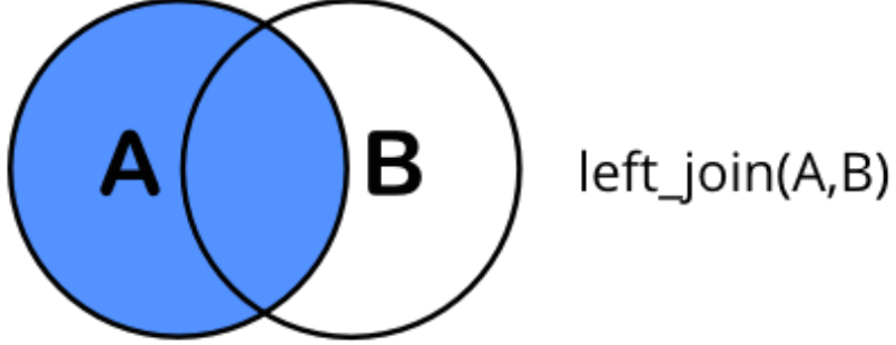
left_join(x, y): all rows from x

## by = keys
left_join(x, y, by = "id")

# A tibble: 3 × 3
     id var_x var_y
  <dbl> <chr> <chr>
1     1 x1    y1   
2     2 x2    y2   
3     3 x3    <NA> 

• NA is added to the id not appearing in y.

• OK first left_join. Look at this gif.
• The idea is that left_join(x, y) keeps all the rows or observations from x, and keep all the variables in x and y, including id, var_x and var_y.
• The variables used to connect two data tables are called keys, and we use by argument to tell dplyr which variable is the key
• By default, the function uses all variables that appear in both tables as keys. So here, the default key is also “id” because “id” is the only variable that appears in both data sets.
• The resulting data frame is shown here. The left join function basically keeps the entire data set x, and attaches the data set y to x with “id” in x.
• Because y doesn’t have id 3, its value of var_y is a missing value NA.
• We can use the venn diagram to visualize the idea of joining tables. And basically, the main data set is A or x. We keep everything of A, and we add stuff of B or y for observations that are in A or x only.

left_join() Example

• Left join
• Code for generating the data sets

pop_x

       state population
1    Alabama    4779736
2     Alaska     710231
3    Arizona    6392017
4   Arkansas    2915918
5 California   37253956
6   Colorado    5029196

elec_vote_y

        state elec_vote
1  California        55
2     Arizona        11
3     Alabama         9
4 Connecticut         7
5      Alaska         3
6    Delaware         3

pop_x |> 
    left_join(elec_vote_y) #<<

       state population elec_vote
1    Alabama    4779736         9
2     Alaska     710231         3
3    Arizona    6392017        11
4   Arkansas    2915918        NA
5 California   37253956        55
6   Colorado    5029196        NA

• Connecticut and Delaware in elec_vote_y will not be shown in the left-joined data because they are not in pop_x.

library(tidyverse)
library(dslabs)
pop_x <- murders |> 
    slice(1:6) |>
    select(state, population)

elec_vote_y <- results_us_election_2016 |> 
    filter(state %in% c("Alabama", "Alaska", "Arizona", 
                        "California", "Connecticut", "Delaware")) |> 
    select(state, electoral_votes) |> 
    rename(elec_vote = electoral_votes)

• Let’s see an example. Here we have two data sets, pop_x and elec_vote_y.
• The left_join() function uses the common variable “state” to combine the two data sets.
• And the result of left joining will be that we keep the entire data set pop_x, and attach the variable elec_vote to the data.
• If there is no such state or observation in y, its corresponding value of elec_vote is NA.

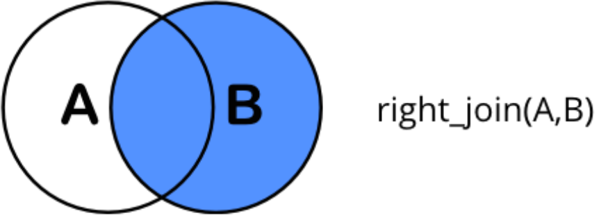
right_join(x, y): all rows from y

right_join(x, y)

Joining with `by = join_by(id)`

# A tibble: 3 × 3
     id var_x var_y
  <dbl> <chr> <chr>
1     1 x1    y1   
2     2 x2    y2   
3     4 <NA>  y4   

• NA is in the column coming from x.

• OK. If you get the idea of left_join, you =should be able to guess what right_join() function is doing.
• Basically right_join(x, y) keeps all the rows or observations from y, and second data set, and again keep all the variablesin both x and y, including id, var_x and var_y.
• For any observation that is not in x, its corresponding value of var_x becomes a missing value NA.
• So here because x does not have id 4, its value of var_x is NA.
• In the venn diagram, the main data set is B or y. We keep everything of B, and we add stuff of A or x for observations that are in B or y only.

right_join() Example

pop_x

       state population
1    Alabama    4779736
2     Alaska     710231
3    Arizona    6392017
4   Arkansas    2915918
5 California   37253956
6   Colorado    5029196

elec_vote_y

        state elec_vote
1  California        55
2     Arizona        11
3     Alabama         9
4 Connecticut         7
5      Alaska         3
6    Delaware         3

pop_x |> 
    right_join(elec_vote_y) #<<

        state population elec_vote
1     Alabama    4779736         9
2      Alaska     710231         3
3     Arizona    6392017        11
4  California   37253956        55
5 Connecticut         NA         7
6    Delaware         NA         3

• Arkansas and Colorado in pop_x will not be shown in the right-joined data because they are not in elec_vote_y.

• Back to the example, if we are doing right-join, we keep the entire data set elec_vote_y, and attach the variable population of pop_x to the data.
• If there is no such state or observation in x, its corresponding value of population is NA.
• Since x does not have Connecticut and Delaware, their population is NA.
• Arkansas and Colorado in pop_x will not be shown in the right-joined data because they are not in elec_vote_y.

full_join(x, y): all rows from both x and y

full_join(x, y)

Joining with `by = join_by(id)`

# A tibble: 4 × 3
     id var_x var_y
  <dbl> <chr> <chr>
1     1 x1    y1   
2     2 x2    y2   
3     3 x3    <NA> 
4     4 <NA>  y4   

• Keep all the rows and fill the missing parts with NAs.

• The next is full_join(). full_join() preserves all the rows or observations either in x or in y or in both x and y.
• In x, we have 1, 2, 3, and in y, we have 1, 2, 4. So the resulting full-joined data frame will have observations 1, 2, 3, 4, and fill the missing parts with NAs.
• x does not have id 4, so its var_x is NA. y does not have id 3, so its var_y is NA

full_join() Example

pop_x

       state population
1    Alabama    4779736
2     Alaska     710231
3    Arizona    6392017
4   Arkansas    2915918
5 California   37253956
6   Colorado    5029196

elec_vote_y

        state elec_vote
1  California        55
2     Arizona        11
3     Alabama         9
4 Connecticut         7
5      Alaska         3
6    Delaware         3

pop_x |> 
    full_join(elec_vote_y) #<<

        state population elec_vote
1     Alabama    4779736         9
2      Alaska     710231         3
3     Arizona    6392017        11
4    Arkansas    2915918        NA
5  California   37253956        55
6    Colorado    5029196        NA
7 Connecticut         NA         7
8    Delaware         NA         3

• full_join() takes the union of observations of x and y, so it produces the data set with the most rows.

• In this example, the full-joined data set will contain observations either in x or in y or in both x and y.
• Because Arkansas and Colorado are not in elec_vote_y, their elec_vote value is NA
• Because Connecticut and Delaware are not in pop_x, their population value is NA
• full_join() takes the union of x and y, so it produces the data set with the most rows.

inner_join(x, y): only rows w/ keys in both x and y

inner_join(x, y)

Joining with `by = join_by(id)`

# A tibble: 2 × 3
     id var_x var_y
  <dbl> <chr> <chr>
1     1 x1    y1   
2     2 x2    y2   

• Keep only the rows that have information in both tables.

• OK inner_join(). inner_join() preserves only rows with keys or id here in both x and y.
• And we know id 1 and id 2 are in both x and y, so these two observations are preserved.
• id 3 is in x, but not in y, id 4 is in y, but not in x, so both are not included in the data.
• Because we are taking intersection of the rows of x and y, we will get the fewest rows when inner_join() is used.

inner_join() Example

pop_x

       state population
1    Alabama    4779736
2     Alaska     710231
3    Arizona    6392017
4   Arkansas    2915918
5 California   37253956
6   Colorado    5029196

elec_vote_y

        state elec_vote
1  California        55
2     Arizona        11
3     Alabama         9
4 Connecticut         7
5      Alaska         3
6    Delaware         3

pop_x |> 
    inner_join(elec_vote_y) #<<

       state population elec_vote
1    Alabama    4779736         9
2     Alaska     710231         3
3    Arizona    6392017        11
4 California   37253956        55

• In this example, there are 4 states in both x and y, Alabama, Alaska, Arizona, and California.
• The inner-joined data set only keep the 4 states data.

16-Joining tables

In lab.qmd ## Lab 16 section

• Import the data at https://www.jaredlander.com/data/DiamondColors.csv. Call it diamond_color.

diamond_color <- readr::read_csv("the url")

• Use left_join() to combine the data set diamonds in ggplot2 and diamond_color by the key variable color.

• Select the variables carat, color, Description, Details.

## Variable "color" in diamonds but "Color" in diamond_color

joined_df <- diamonds |>  
    _______(_______, by = c('color' = 'Color')) |>  ## join
    _______(_________________________________________)  ## select

• Create a bar chart of the variable color.

# A tibble: 53,940 × 4
  carat color Description    Details                  
  <dbl> <chr> <chr>          <chr>                    
1  0.23 E     Colorless      Minute traces of color   
2  0.21 E     Colorless      Minute traces of color   
3  0.23 E     Colorless      Minute traces of color   
4  0.29 I     Near Colorless Slightly detectable color
5  0.31 J     Near Colorless Slightly detectable color
6  0.24 J     Near Colorless Slightly detectable color
# ℹ 53,934 more rows

Joining Data Frames

pd.merge()

pd.merge()

• Left join
• Code for generating the data sets

import numpy as np
import pandas as pd

pop_x

        state  population
0     Alabama     4779736
1      Alaska      710231
2     Arizona     6392017
3    Arkansas     2915918
4  California    37253956
5    Colorado     5029196

elec_vote_y

          state  electoral_votes
21      Alabama                9
43       Alaska                3
13      Arizona               11
0    California               55
26  Connecticut                7
44     Delaware                3

## dplyr::left_join()
pd.merge(pop_x, elec_vote_y, how = 'left')

        state  population  electoral_votes
0     Alabama     4779736              9.0
1      Alaska      710231              3.0
2     Arizona     6392017             11.0
3    Arkansas     2915918              NaN
4  California    37253956             55.0
5    Colorado     5029196              NaN

murders = pd.read_csv('./data/murders.csv')
pop_x = murders[0:6][['state','population']]

election = pd.read_csv('./data/results_us_election_2016.csv')
raws1 = ["Alabama", "Alaska", "Arizona", "California", "Connecticut", "Delaware"]
cols1 = ["state", "electoral_votes"]
df = election[cols1]
pop = []
for i in raws1:
    mask = df["state"] == i
    pos = np.flatnonzero(mask)
    pop.append(pos)

pop = np.array(pop)
pop = np.resize(pop, 6)
elec_vote_y = df.iloc[pop]

pd.merge(pop_x, elec_vote_y, how = 'right') ## dplyr::right_join()

         state  population  electoral_votes
0      Alabama   4779736.0                9
1       Alaska    710231.0                3
2      Arizona   6392017.0               11
3   California  37253956.0               55
4  Connecticut         NaN                7
5     Delaware         NaN                3

pd.merge(pop_x, elec_vote_y, how = 'outer') ## dplyr::full_join()

         state  population  electoral_votes
0      Alabama   4779736.0              9.0
1       Alaska    710231.0              3.0
2      Arizona   6392017.0             11.0
3     Arkansas   2915918.0              NaN
4   California  37253956.0             55.0
5     Colorado   5029196.0              NaN
6  Connecticut         NaN              7.0
7     Delaware         NaN              3.0

pd.merge(pop_x, elec_vote_y, how = 'inner') ## dplyr::inner_join()

        state  population  electoral_votes
0     Alabama     4779736                9
1      Alaska      710231                3
2     Arizona     6392017               11
3  California    37253956               55