Linear Regression

MATH/COSC 3570 Introduction to Data Science

Dr. Cheng-Han Yu
Department of Mathematical and Statistical Sciences
Marquette University

What is Regression

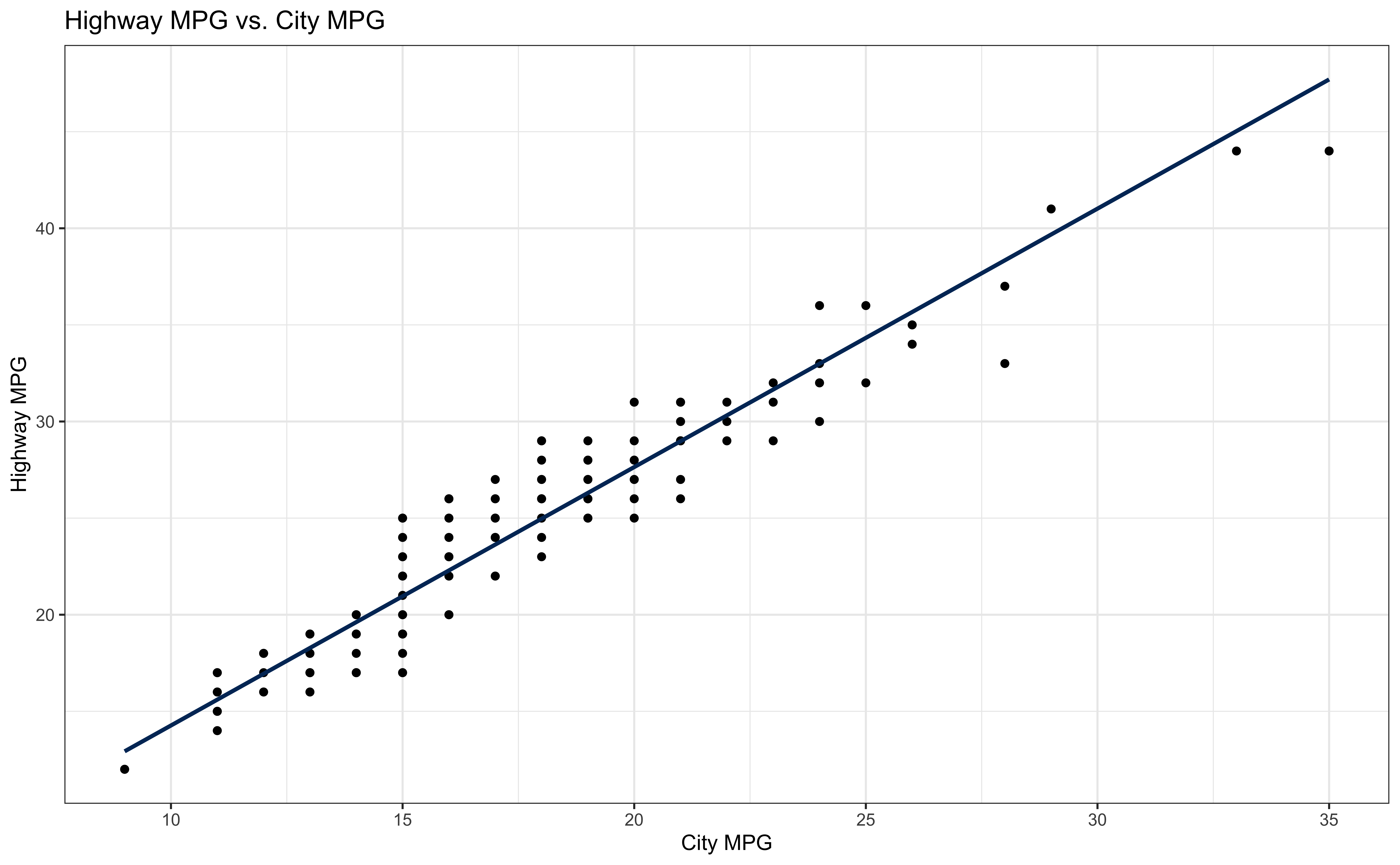
• Regression models the relationship between a numerical response variable \((Y)\) and one or more numerical/categorical predictors \((X)\), which is a supervised learning method in machine learning.

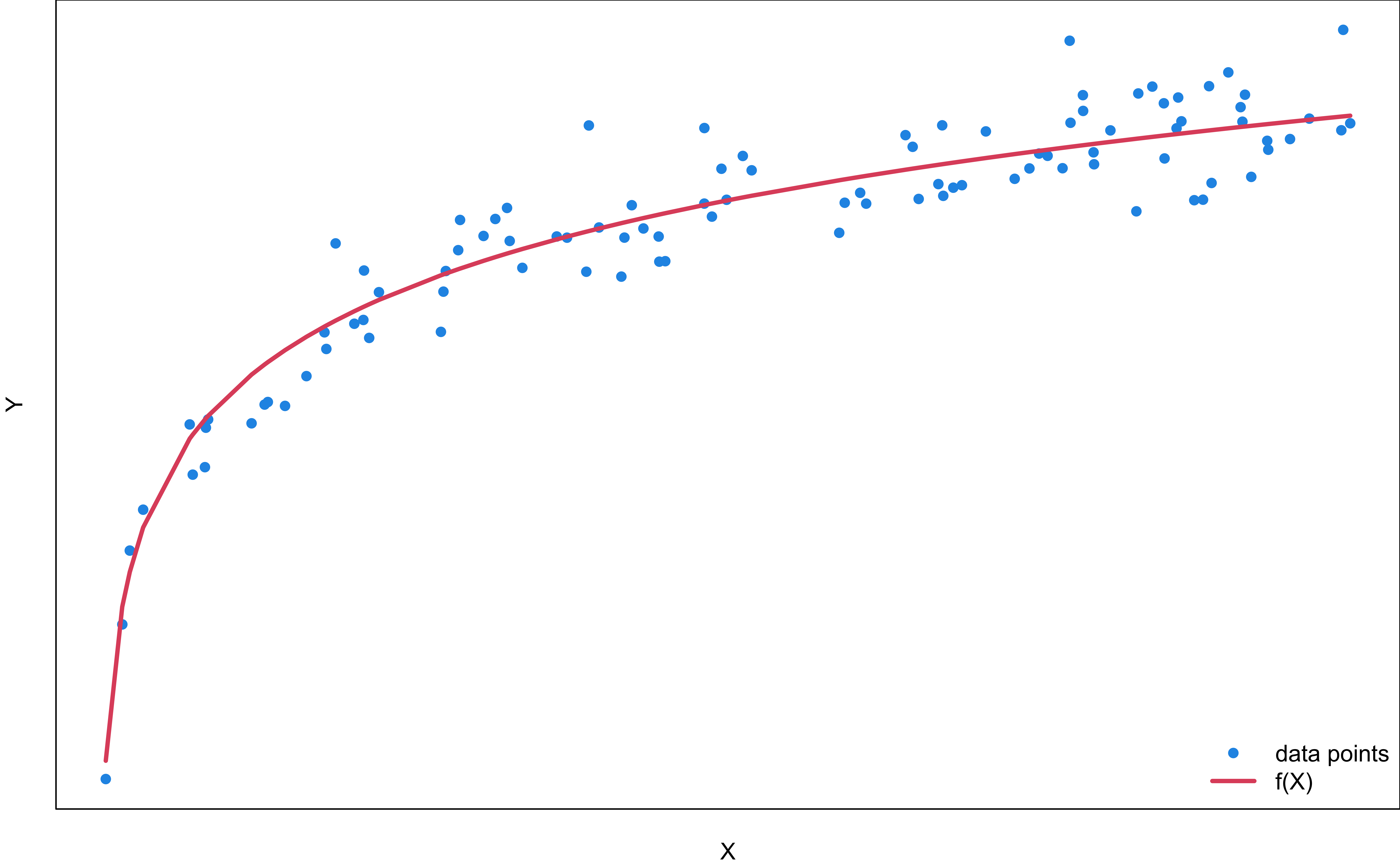
• A regression function \(f(X)\) describes how a response variable \(Y\) generally changes as an explanatory variable \(X\) changes.

Examples:

• college GPA \((Y)\) vs. ACT/SAT score \((X)\)

• sales \((Y)\) vs. advertising expenditure \((X)\)

• crime rate \((Y)\) vs. median income level \((X)\)

Simple Linear Regression

\[\begin{align*} y_i &= f(x_i) + \epsilon_i \\ &= \beta_0 + \beta_1~x_{i} + \epsilon_i, \quad i = 1, 2, \dots, n \end{align*}\]

• \(\beta_0\) and \(\beta_1\) are unknown parameters to be learned or estimated.

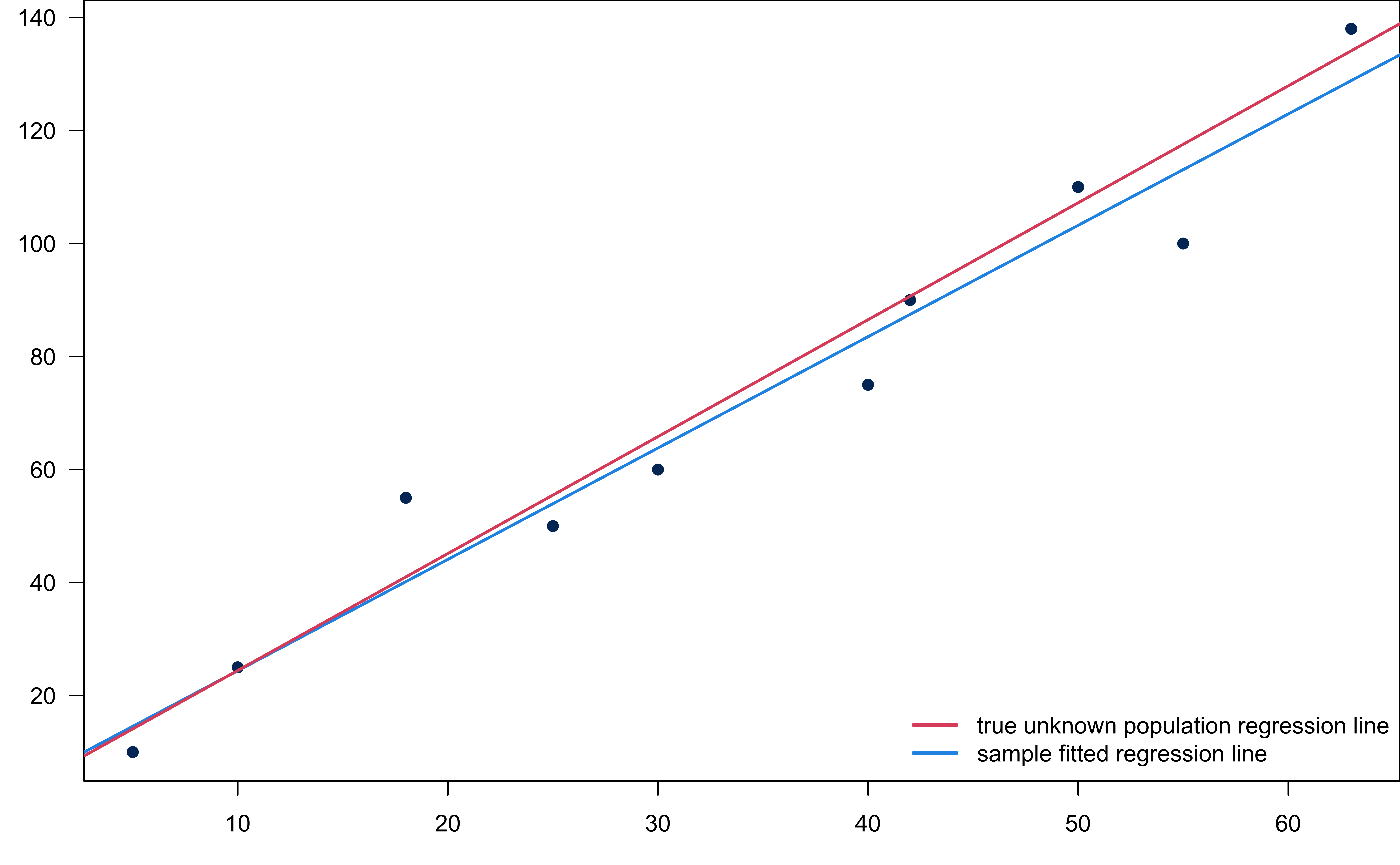
What are the assumption on \(\epsilon_i\)?

\(\epsilon_i \sim N(0, \sigma^2)\) and hence \(y_i \mid x_i \sim N(\beta_0+\beta_1x_i, \sigma^2)\)

• OK we start with the simple linear regression, the linear regression a Single Predictor \(x\).
• In linear regression, our regression function \(f\) is a linear function \(\beta_0 + \beta_1~x\).
• Epsilon, the random error is there to capture any random measurement errors or any variations in \(y\) that cannot be explained by the predictor \(x\).
• Given this model, we’re interested in \(\beta_0\) (population parameter for the intercept) and \(\beta_1\) (population parameter for the slope) because once we know \(\beta_0\) and \(\beta_1\), we know the exact shape of \(f\) and we know the relationship of \(y\) and \(x\), and given any value of \(x\), we can predict its corresponding value of \(y\) using the regression line \(\hat{y}_{i} = \beta_0 + \beta_1~x_{i}\).
• But unfortunately, the population parameters are typically unknown to us.

Simple Linear Regression Assumptions

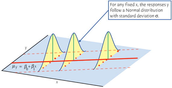
Simple Linear Regression Assumptions

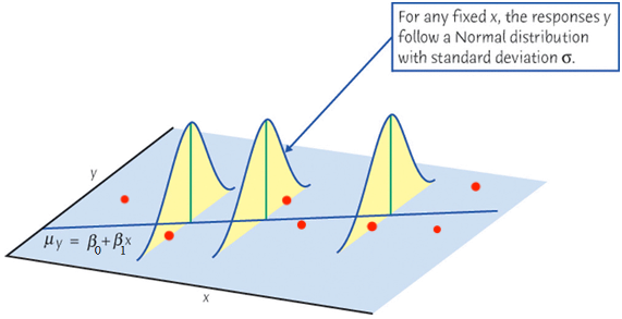
Simple Linear Regression Assumptions

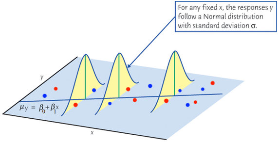
Ordinary Least Squares (OLS)

Given the training data \((x_1, y_1), \dots, (x_n, y_n)\), use sample statistics \(b_0\) and \(b_1\) computed from the data to

• inference: estimate \(\beta_0\) and \(\beta_1\)

• fitting: estimate \(y_i\) or \(f(x_i)\) at \(x_i\) by its fitted value \[\hat{y}_{i} = \hat{f}(x_i) = b_0 + b_1~x_{i}\]

• prediction: predict \(y_j\) or \(f(x_j)\) at \(x_j\) by its predicted value \[\hat{y}_{j} = \hat{f}(x_j) = b_0 + b_1~x_{j}\] where \((x_j, y_j)\) is never seen and used in training before.

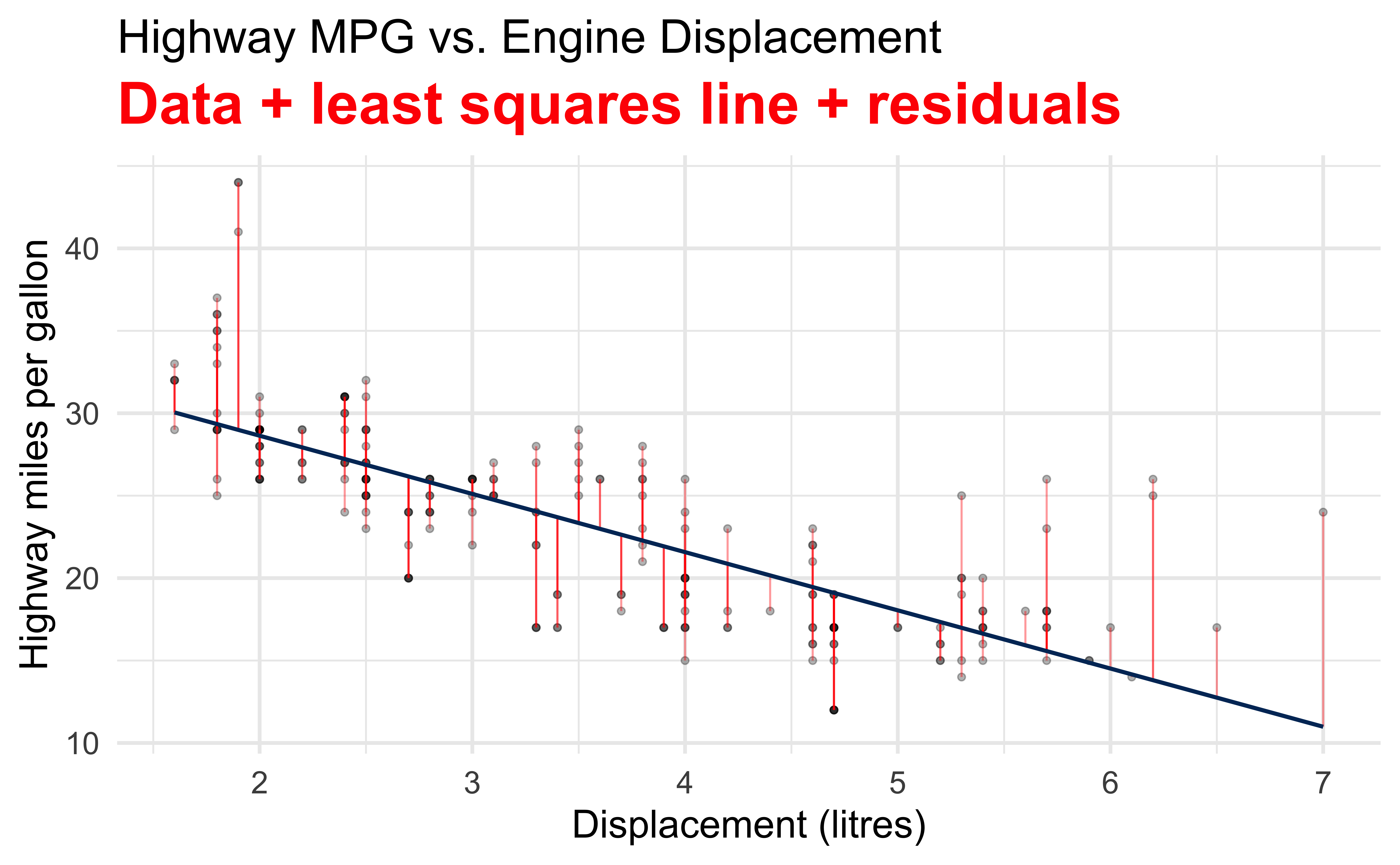
• Ordinary Least Squares: Find \(b_0\) and \(b_1\), or regression line \(b_0 + b_1x\) that minimizes the sum of squared residuals.
• The residual \(e_i = y_i - \hat{y}_i\). The sample regression line minimizes \(\sum_{i = 1}^n e_i^2\).

• How do we get \(b_0\) and \(b_1\) that sort of well estimate \(\beta_0\) and \(\beta_1\)?
• We choose \(b_0\) and \(b_1\), or regression line \(b_0 + b_1x\) that minimizes the sum of squared residuals.
• If we define residual as \(e_i = y_i - \hat{y}_i\), then the sum of squared residuals is \(\sum_{i = 1}^n e_i^2\).
• And this approach that estimates the population parameters \(\beta_0\) and \(\beta_1\) or the population regression line is called Ordinary Least Squares method.

Visualizing Residuals

OK. That’s see the idea of Ordinary Least Squares visually. Here just showed the data. - Do you see why some points are darker than some others? - A darker point means that there are several identical (x, y) pairs, or replicates in the data set.

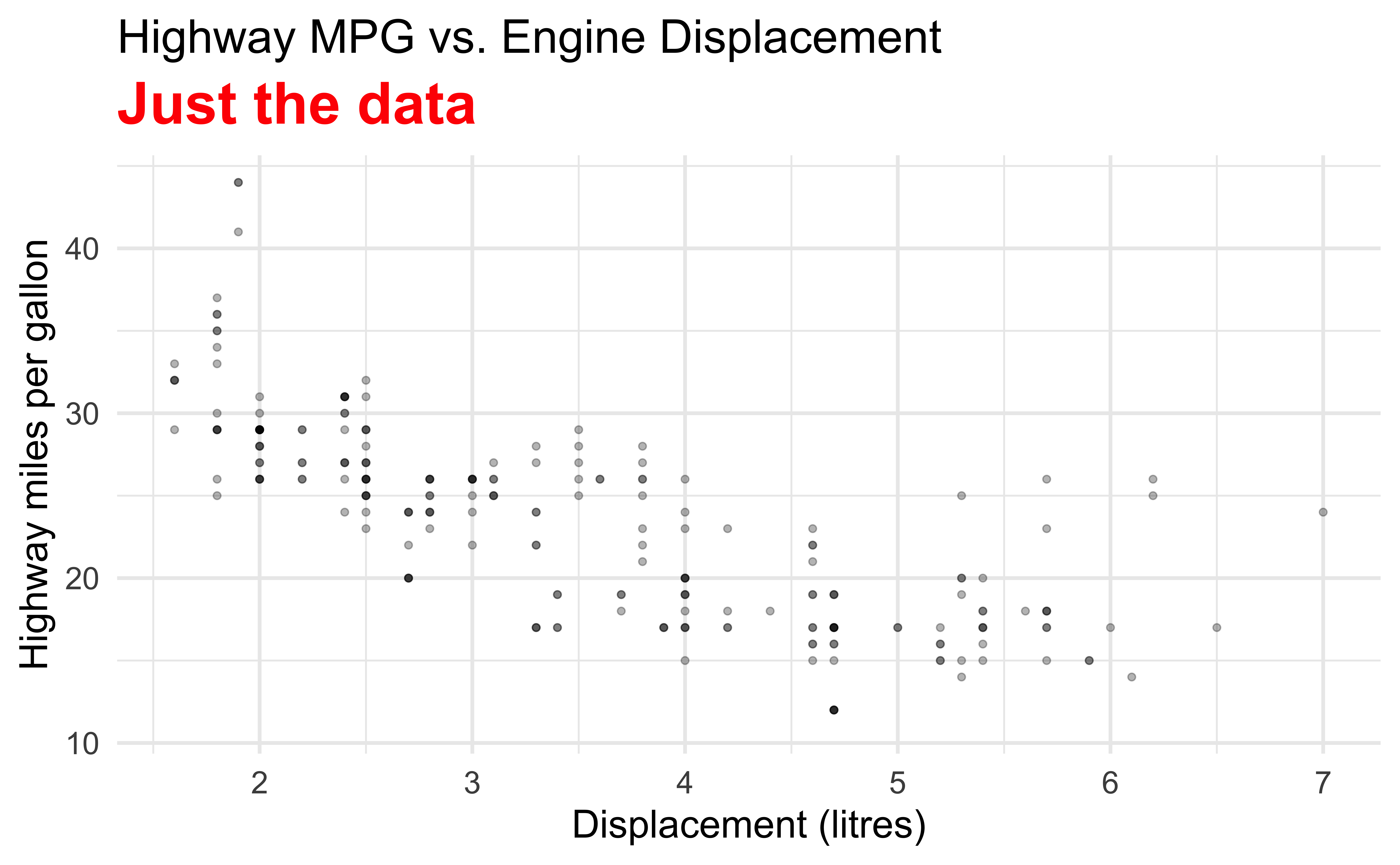
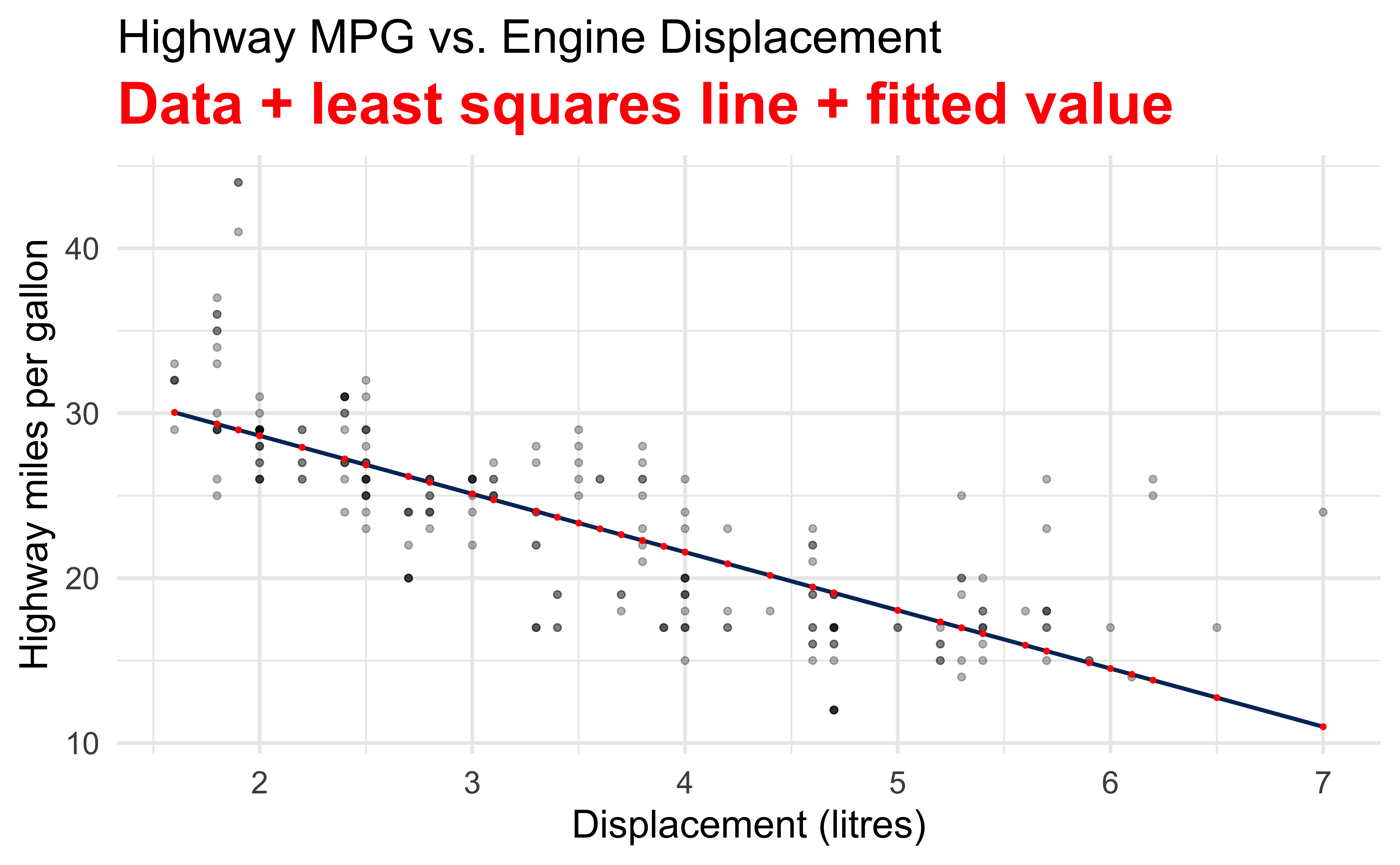
Visualizing Residuals (cont.)

• All right, with the data, this figure also shows the least squares regression line, and the fitted (predicted) value of \(y\) for each \(x\) in the training data, which are those red points.
• The predicted values of y are right on the regression line.
• Now the question is, how do we find this line?
• Given a line, we can have predicted values of y, right?
• Then what is residual on the plot? The residual will be the difference between the true observation y and the predicted value of y given any value of x.
• So a residual in the plot will be a vertical bar at the value of x with two ends of the bar \(y\) and \(\hat{y}\), right?
• (Show on board)
• (add \(y_i = b_0+b_1x_i\) and residual line)

Visualizing Residuals (cont.)

• Here shows all the residuals in vertical bars.
• least squares line is the line such that the sum of all the squared residuals is minimized.
• Why we square the residuals?
• It’s mathematically more convenient.
• Squaring emphasizes larger differences

Fitting and Interpreting Regression Models

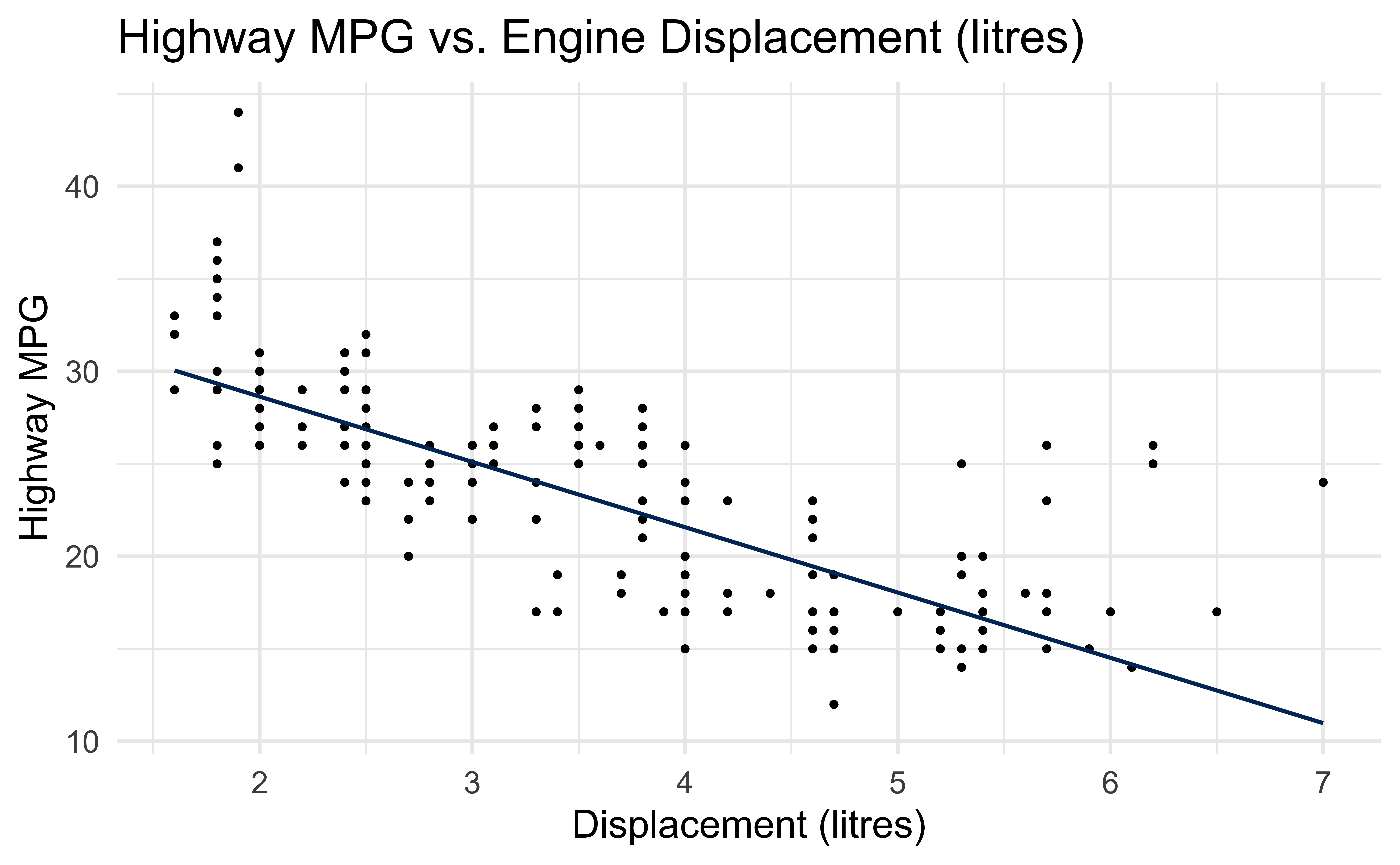
Predict Highway MPG hwy from Displacement displ

\[\widehat{hwy}_{i} = b_0 + b_1 \times displ_{i}\]

• The data I just show you is the mpg data set in ggplot2.
• Here we are trying to Predict Highway MPG hwy from Engine Displacement displ

Tidymodels

Step 1: Specify Model: linear_reg()

library(tidymodels)
parsnip::linear_reg()

Linear Regression Model Specification (regression)

Computational engine: lm 

parsnip package provides a tidy, unified interface for fitting models

One challenge with different modeling functions available in R that do the same thing is that they can have different interfaces and arguments. Note that the model syntax can be very different and that the argument names (and formats) are also different. This is a pain if you switch between implementations. - So how do we use tidymodels to actually fit a model. - Step 1 is to specify the model that we are building. - We are going to build a linear regression model, so the function we start with is linear_reg() - And you can see that the output is saying OK I’m ready to use this model specification.

Step 2: Set Model Fitting Engine

• By default, use lm() in the built-in stats package.

linear_reg() |> 
    set_engine("lm")

Linear Regression Model Specification (regression)

Computational engine: lm 

show_engines("linear_reg")

# A tibble: 7 × 2
  engine mode      
  <chr>  <chr>     
1 lm     regression
2 glm    regression
3 glmnet regression
4 stan   regression
5 spark  regression
6 keras  regression
7 brulee regression

• Step 2 is to define the model fitting engine.
• For now we are going to use “lm” that is a function in the stats package to fit a linear model.
• Basically, we ask R or tidymodel to use the lm() function as our computational engine to fit a linear regression model.
• So you can think tidymodel as an platform or interface with many other R packages that do the work of model fitting, and tidymodel provides a consistent interface to them.
• So you can actually use different R packages as different computational engines to fit the same model.
• With tidymodel, you don’t need to worry about different syntax should be used in different packages because the syntax is the same, and its outputs also remain the same even different computational engine is used.

Step 3: Fit Model & Estimate Parameters

… using formula syntax

linear_reg() |> 
    fit(hwy ~ displ, data = mpg)

parsnip model object


Call:
stats::lm(formula = hwy ~ displ, data = data)

Coefficients:
(Intercept)        displ  
      35.70        -3.53  

\[\widehat{hwy}_{i} = 35.7 -3.53 \times displ_{i}\]

• Slope: When the engine displacement volume of a car is increased by one litre, the highway miles per gallon is expected to be lower, on average, by 3.53 miles.

• Step 3, after selecting the computational engine, we fit the model and estimate parameters.
• we use the fit() function, and inside the function, we provide the model fitting formula, response variable ~ predictors, followed by the data set’s name.
• Here our response is hwy, and the predictor is displ, and the data set is mpg.
• After fitting the model, we can the model output. We can see our estimated coefficients intercept and slope for displ, which are \(b_0\) and \(b_1\) in previous slides.
• And with the coefficients, we now can have the regression line, \(\widehat{hwy}_{i} = 35.698 -3.531 \times displ_{i}\), where \(\widehat{hwy}_{i}\) is the predicted value of hwy MPG of the \(i\)-th observation.

Tidy Look at Model Output

• Tidymodels output (tibble)

linear_reg() |> 
    fit(hwy ~ displ, data = mpg) |> 
    tidy()

# A tibble: 2 × 5
  term        estimate std.error statistic   p.value
  <chr>          <dbl>     <dbl>     <dbl>     <dbl>
1 (Intercept)    35.7      0.720      49.6 2.12e-125
2 displ          -3.53     0.195     -18.2 2.04e- 46

\[\widehat{hwy}_{i} = 35.7 -3.53 \times displ_{i}\]

• We can print the model output as a tidy table using the tidy() function.
• Here we not only have the point estimates in the fist column, but also have the standard error that measure the uncertainty of these coefficients, the test statistics, and p-values that are used in hypothesis testing.
• We’ll use standard error when quantifying the uncertainty about the regression line, but we won’t talk about test statistics and p-values in this course because they are covered in 4720.

20-Simple Linear Regression

In lab.qmd ## Lab 20 section,

• Use the mpg data to fit a simple linear regression where \(y\) is hwy and \(x\) is cty.

• Produce the plot below. (add the layer geom_smooth(method = "lm", se = FALSE))

library(tidymodels); library(ggplot2)

parsnip::linear_reg() %>% 
    set_engine("lm") %>% 
    fit(hwy ~ displ, data = mpg) %>% 
    tidy()

library(tidymodels); library(ggplot2)
ggplot(data = mpg, aes(x = cty, y = hwy)) +
    geom_point() +
    geom_smooth(method = "lm", se = FALSE, color = "#003366") + 
    labs(title = "Highway MPG vs. City MPG",
         x = "City MPG",
         y = "Highway MPG")

Quantify Uncertainty about Coefficients

• Uncertainty about regression coefficients \(\beta_0\) and \(\beta_1\)

reg_out <- linear_reg() |> 
    fit(hwy ~ displ, data = mpg)

reg_out_fit <- reg_out$fit

reg_out_fit$coefficients

(Intercept)       displ 
      35.70       -3.53 

confint(reg_out_fit)

            2.5 % 97.5 %
(Intercept) 34.28  37.12
displ       -3.91  -3.15

Quantify Uncertainty about Mean of \(y\)

• Uncertainty about the mean value of \(y\) given \(X = x\) \[\mu_{Y \mid X = x} = \beta_0 + \beta_1x\]

new_input <- data.frame(displ = 3:6)

predict(reg_out_fit, newdata = new_input, interval = "confidence", level = 0.95)

   fit  lwr  upr
1 25.1 24.6 25.6
2 21.6 21.0 22.1
3 18.0 17.3 18.8
4 14.5 13.4 15.6

• We are also interested in uncertainty about the mean value of \(y\) given some value of \(x\), especially when we are predicting \(y\).
• To get the CI for the mean of \(y\) at any value of \(x\), we can use the predict() function.
• The first argument in the function is the regression fitted result.
• Then and argument new data is a data frame of predictor values.
• Here, the predictor is at 1, 2, 3, up to 8.
• And interval is confidence, and confidence level is 95%.
• The output will have 3 columns. The first column shows the predicted or fitted value of \(y\) given \(x\), these are values right on the regression line.
• The second and third columns are lower and upper bound respectively.
• How do we show the confidence interval for the mean of y?
• Again we use geom_smooth() layer, and set se = TRUE, so that geom_smooth() uses the standard error info to obtain the confidence interval for us.

Quantify Uncertainty about Mean of \(y\)

• Fit with uncertainty band
• ggplot code

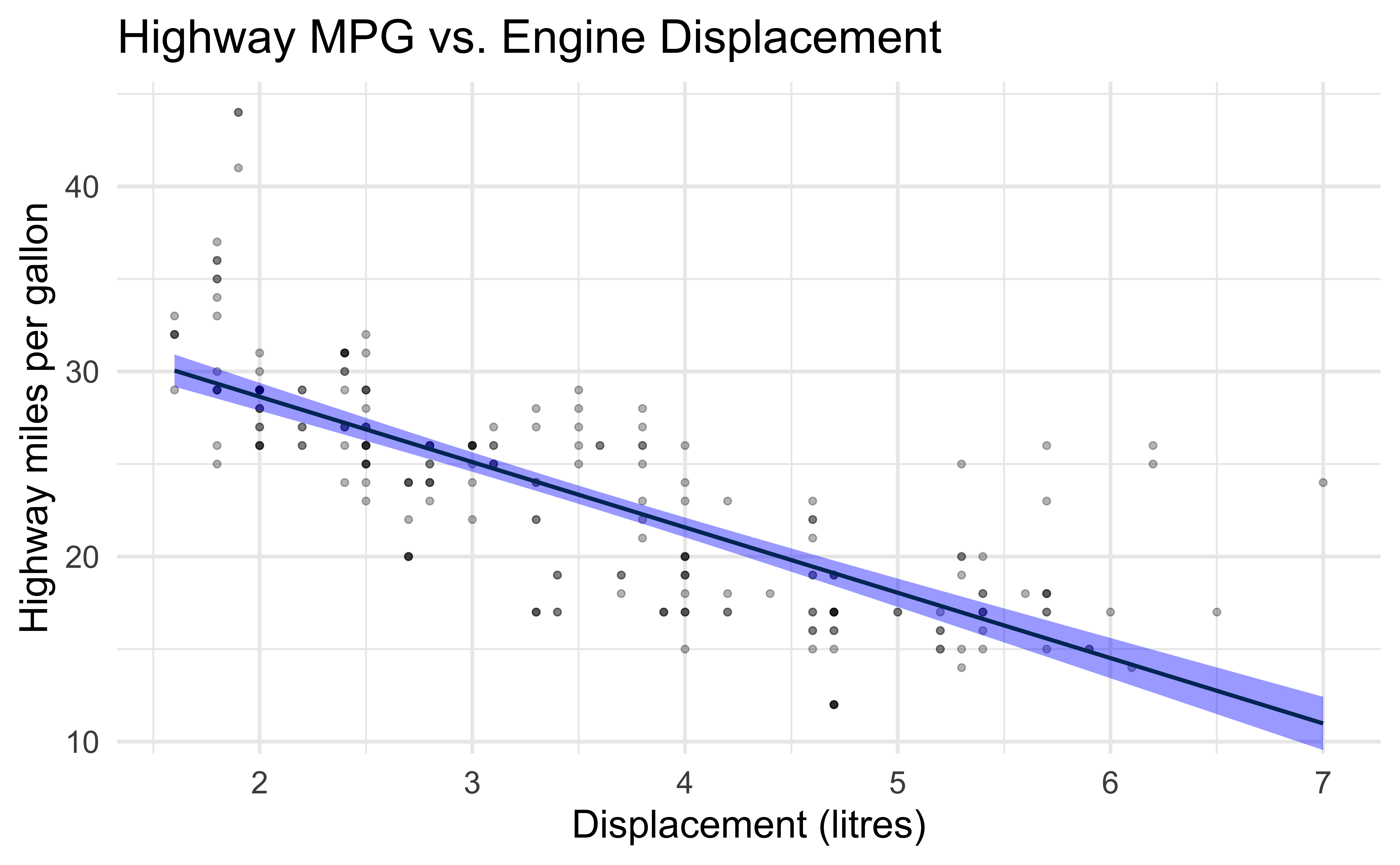
p <- ggplot(data = reg_out_fit, 
            aes(x = displ, y = hwy)) +
     geom_point(alpha = 0.3) + 
     labs(title = "Highway MPG vs. Engine Displacement",
          x = "Displacement (litres)",
          y = "Highway miles per gallon") +
      coord_cartesian(ylim = c(11, 44))

p_ci <- p + geom_smooth(method = "lm", 
                        color = "#003366", 
                        fill = "blue",
                        se = TRUE)

Quantify Uncertainty about Individual \(y\)

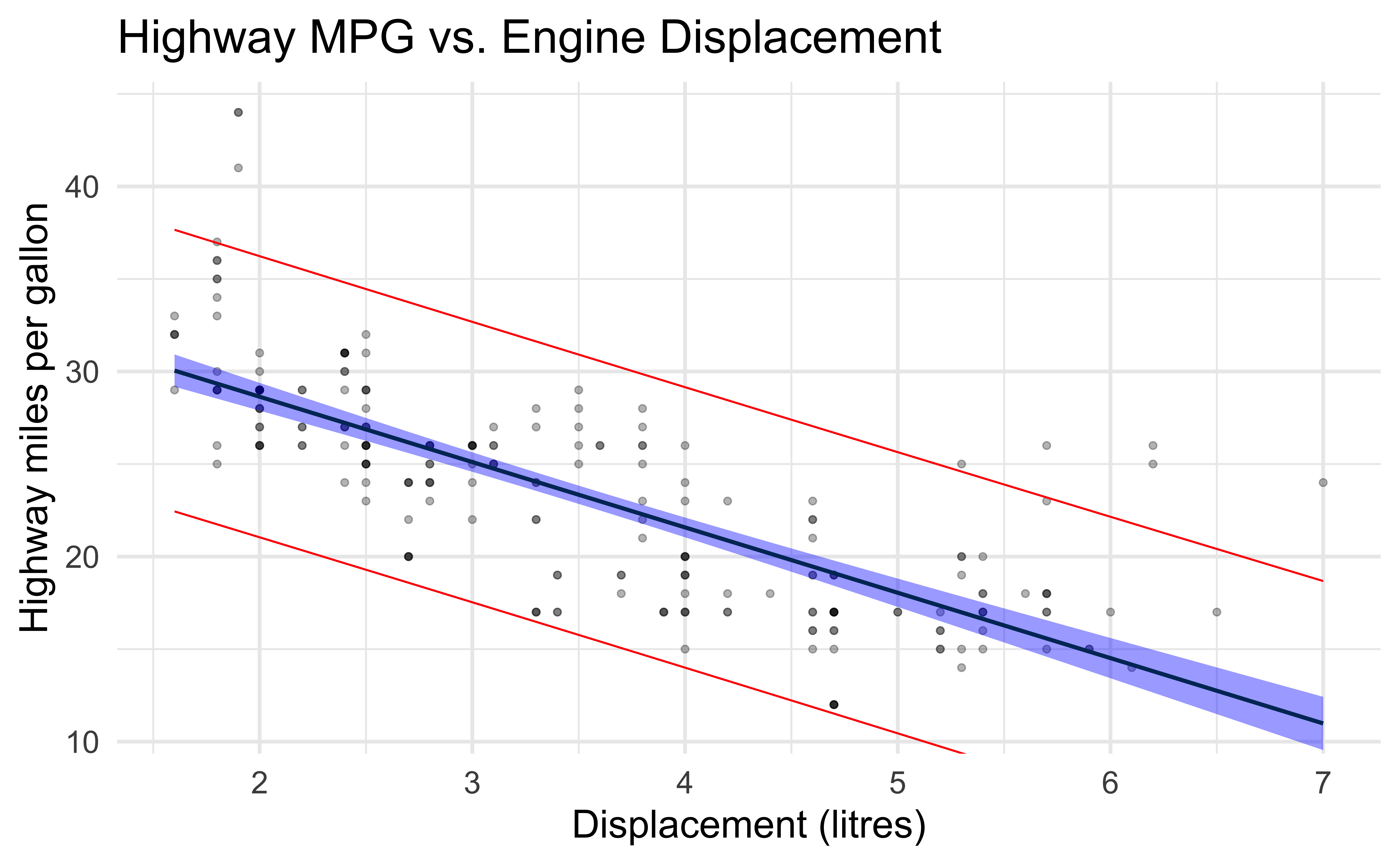
• Uncertainty about the individual value of \(y\) given \(X = x\), \(Y \mid X = x\)

predict(reg_out_fit, newdata = new_input, interval = "prediction", level = 0.95)

   fit   lwr  upr
1 25.1 17.53 32.7
2 21.6 14.00 29.2
3 18.0 10.45 25.6
4 14.5  6.88 22.1

## predict at current inputs
pred_y <- predict(reg_out_fit, interval = "prediction")
head(pred_y)

   fit  lwr  upr
1 29.3 21.7 36.9
2 29.3 21.7 36.9
3 28.6 21.0 36.2
4 28.6 21.0 36.2
5 25.8 18.2 33.4
6 25.8 18.2 33.4

• We can also quantify the uncertainty about the value individual \(y\) given \(x\).
• As you can imagine, this is more difficult to predict value of individual \(y\) than to predict value of mean of \(y\), right?
• Because individual \(y\) value varies more than the mean of \(y\) due to the random error noises added to it.
• And so with the same confidence level, the CI for individual \(y\) will be much wider than the CI for the mean of \(y\).
• How do we get the CI?
• The code is basically the same as before. But here instead of “confidence”, here we use “prediction” in the interval argument.
• You can see that the 95% interval is much wider, trying to capture or contain most of the observed values of \(y\).

Quantify Uncertainty about Individual \(y\)

p_ci + 
    geom_line(aes(x = displ, y = pred_y[, "lwr"]), color = "red") +
    geom_line(aes(x = displ, y = pred_y[, "upr"]), color = "red")

Model Checking

• OK. Model checking. How do we know linear regression model is a good model for fitting our data. Well, we can assess the quality of the model by looking at residuals. Let’s see how.

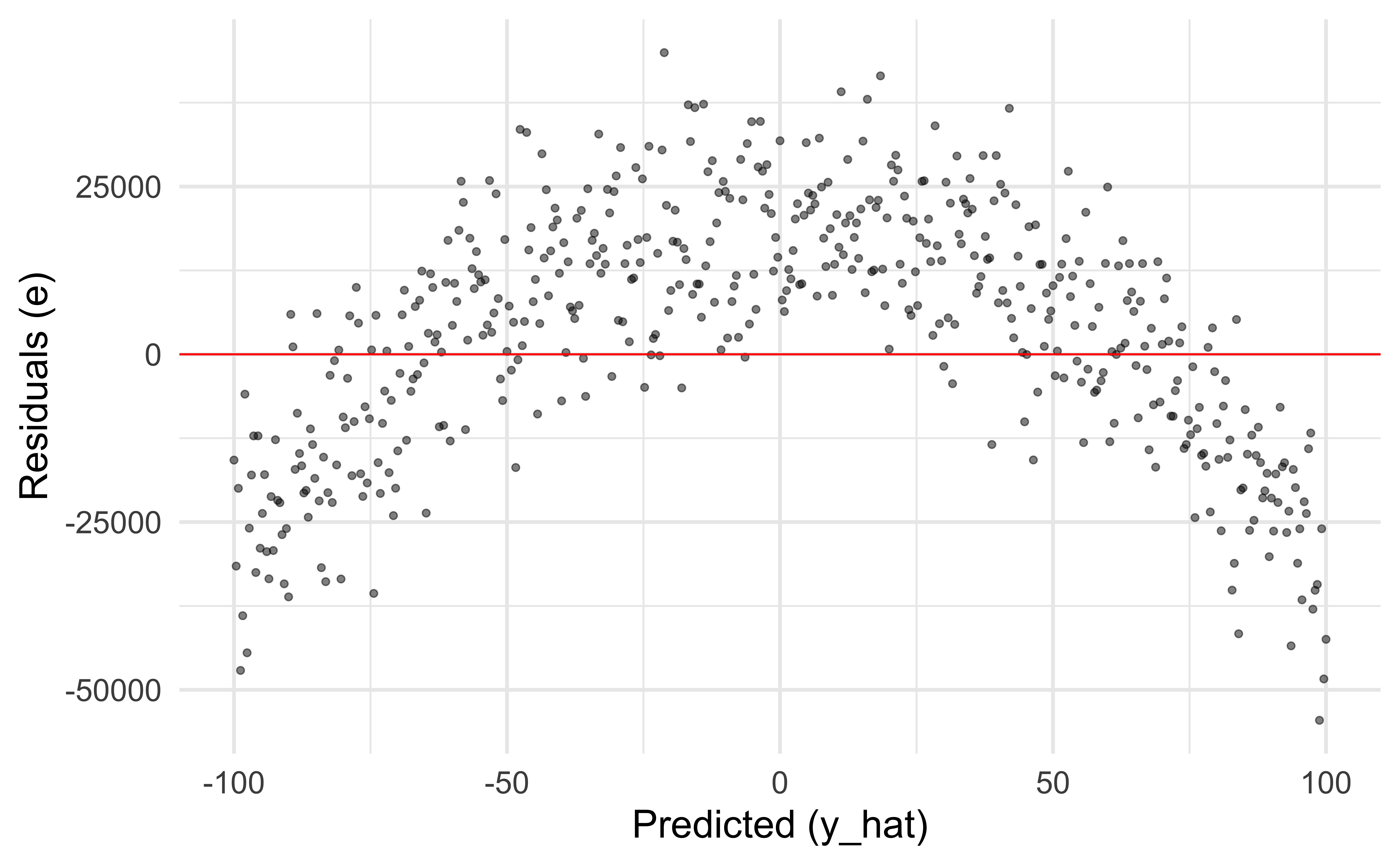
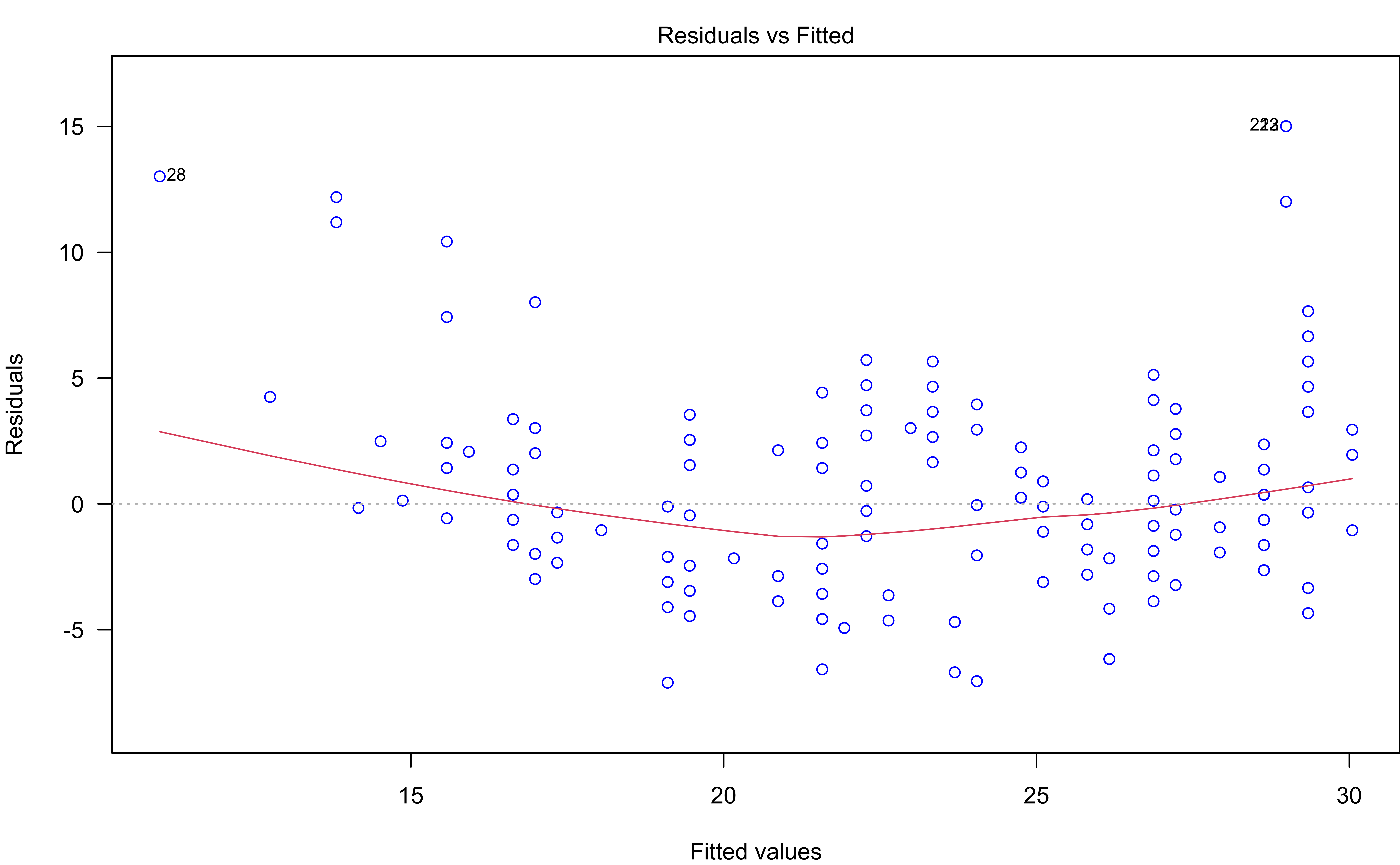
Graphical Diagnostics: Residual Plot

• Residuals distributed randomly around 0.
• Check it by plotting residuals against the fitted value of \(y\): \(e_i\) vs. \(\hat{y}_i\)
• With no visible pattern along the x or y axis.

We are looking for - Residuals distributed randomly around 0. - With no visible pattern along the \(x\) or \(y\) axes. - This can be checked by plotting residuals against the fitted value of \(y\). - Here shows a good residual plot. Residuals are around 0, and its variation is more or less the same across different values of \(\hat{y}\). - There is no significant pattern in the plot.

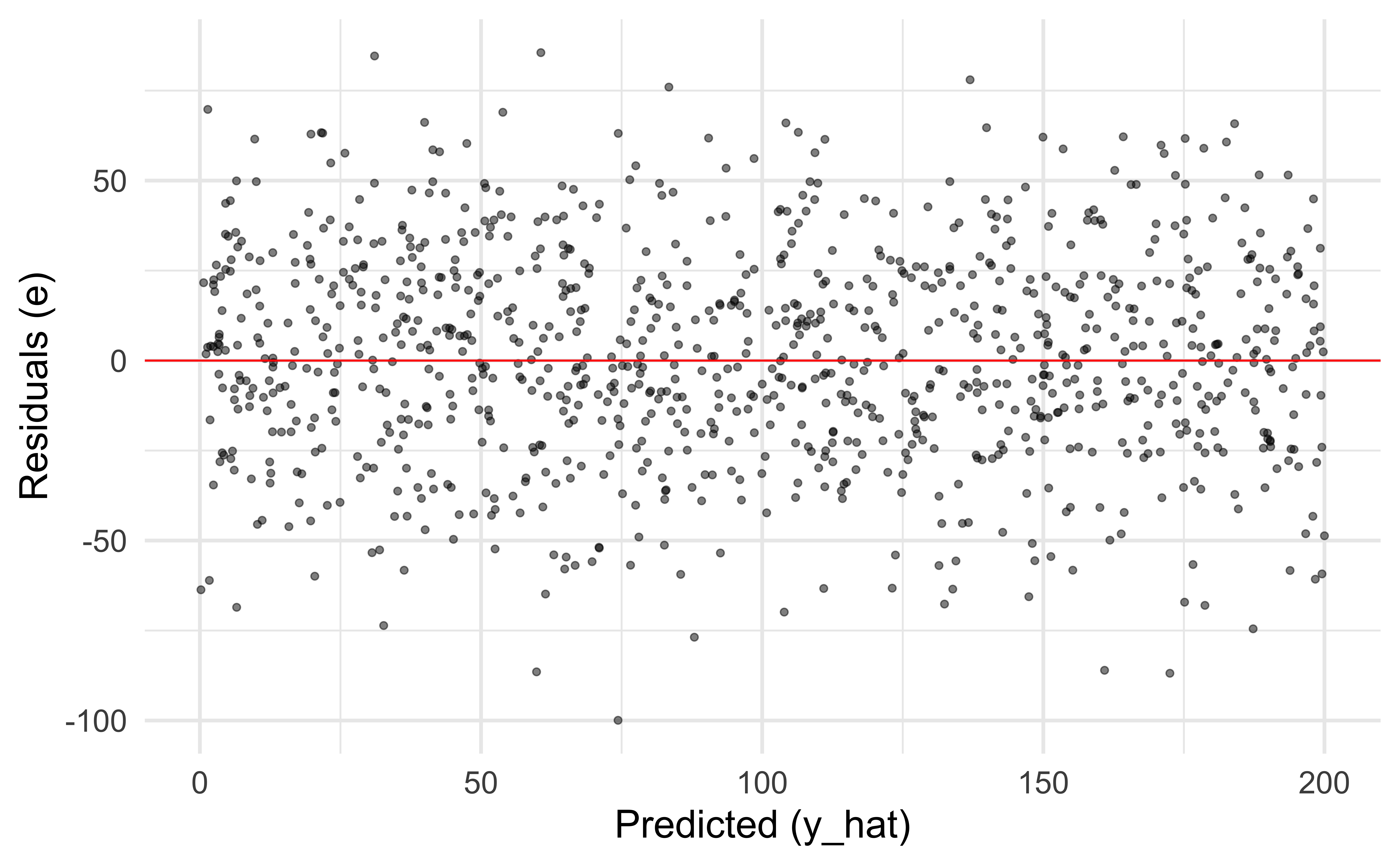
Not looking for…

Fan shapes

• We are not looking for a plot that has a fan shape.

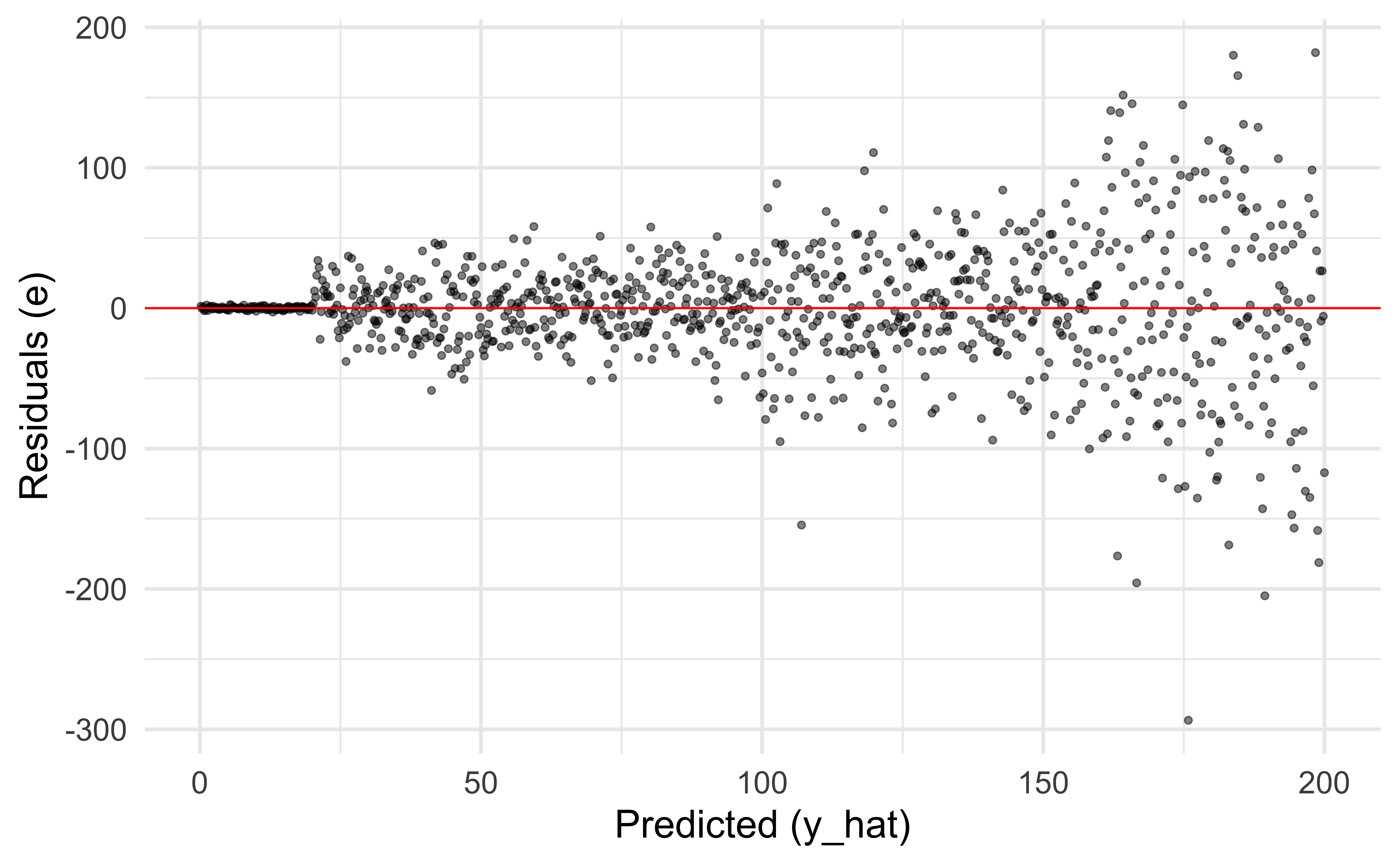
Not looking for…

Groups of patterns

• We are not looking for a plot that has Groups of patterns

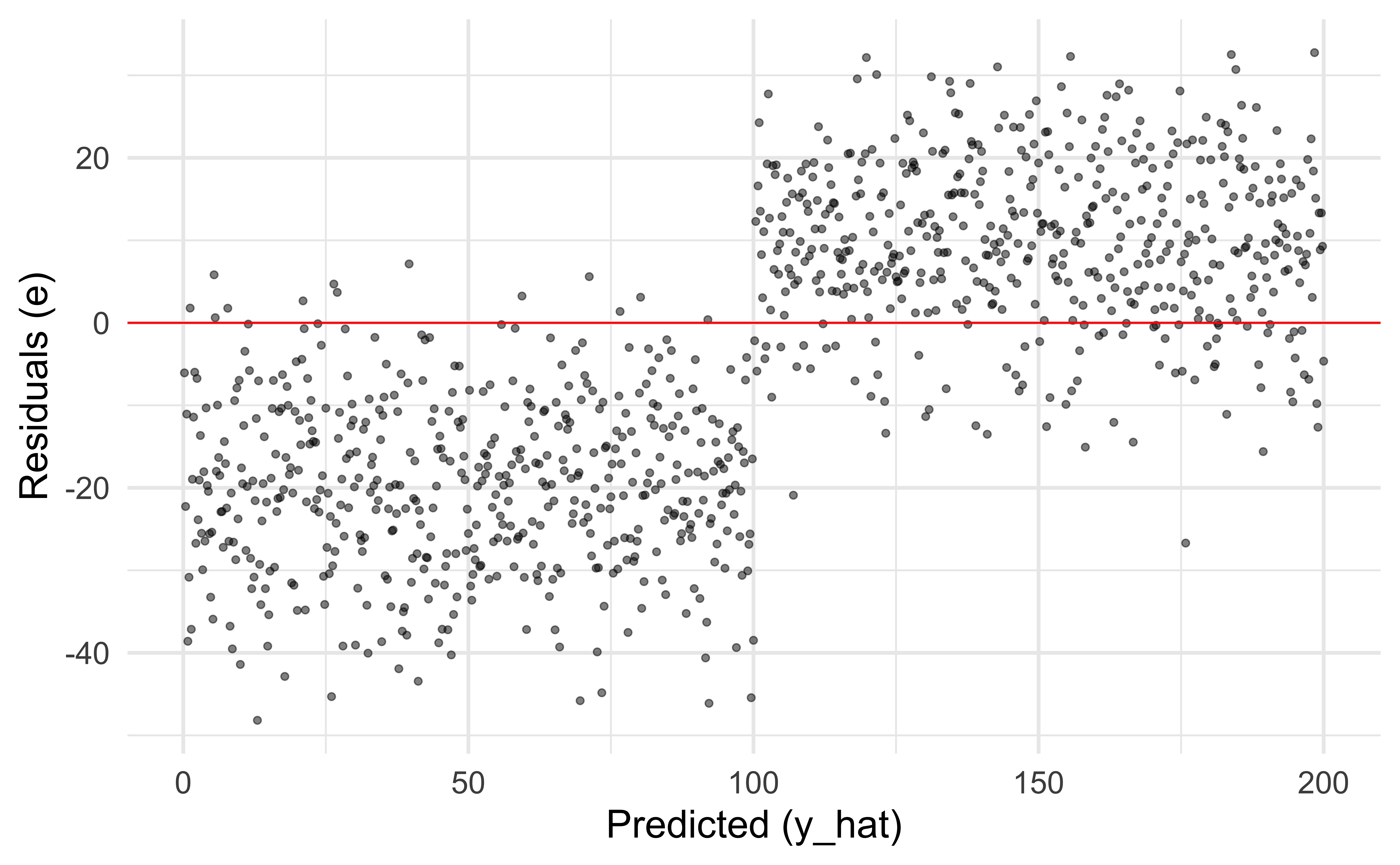
Not looking for…

Residuals correlated with predicted values

• We also don’t want Residuals to be correlated with predicted values

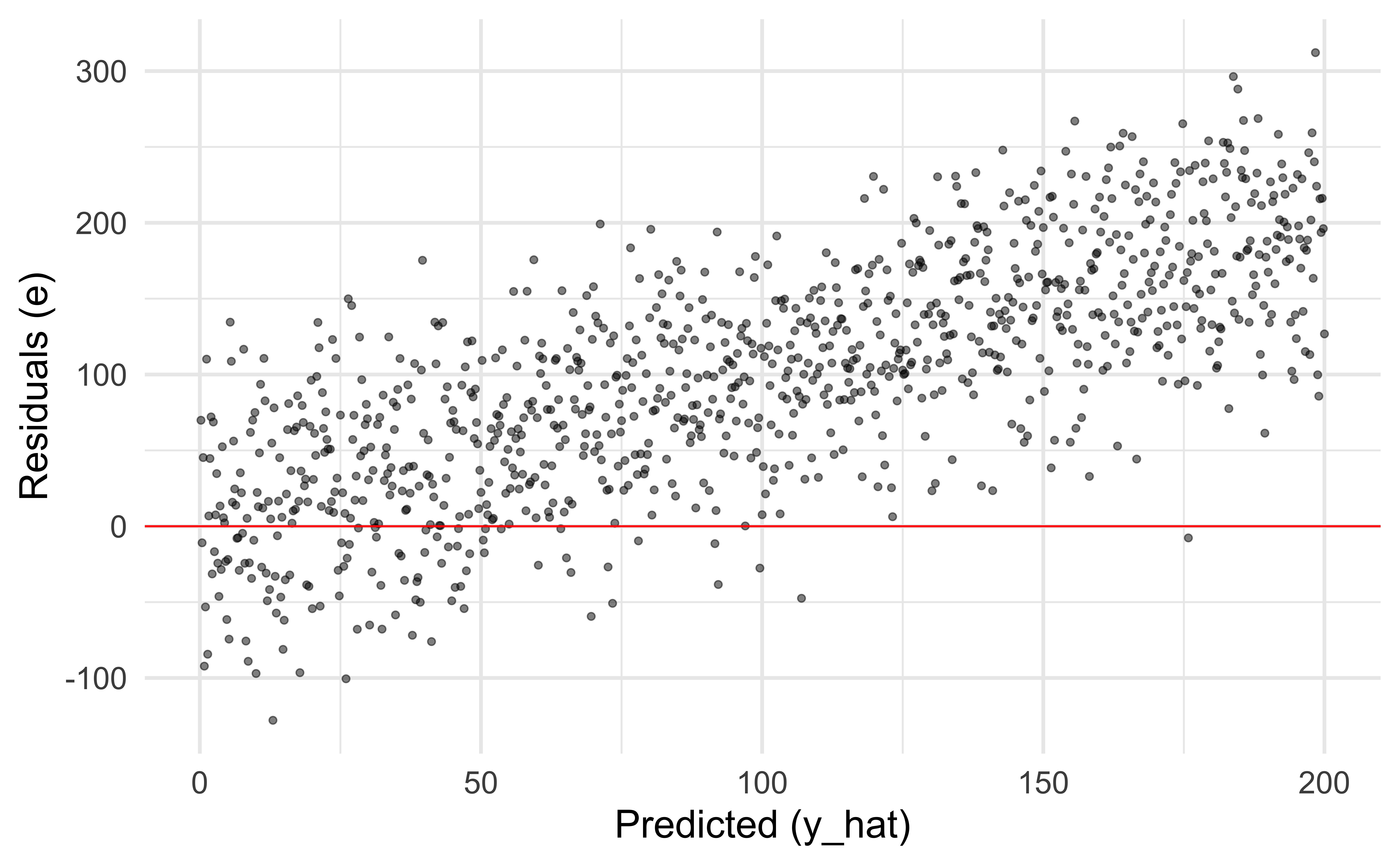
Not looking for…

Any patterns!

• We basically don’t want the residuals show Any patterns!
• If \(X\) and \(Y\) are not linearly related, or the residual plot exists some pattern, some data transformation is needed. Or use another model.

MPG Data Residuals

plot(reg_out_fit, which = 1, col = "blue", las = 1)

Models with Categorical Predictors

Categorical Predictor with 2 Categories

mpg |>  
  select(hwy, trans) |>  
  print(n = 4)

# A tibble: 234 × 2
    hwy trans     
  <int> <chr>     
1    29 auto(l5)  
2    29 manual(m5)
3    31 manual(m6)
4    30 auto(av)  
# ℹ 230 more rows

mpg_new <- mpg
mpg_new$trans[grepl("auto", mpg_new$trans)] <- "auto"
mpg_new$trans[grepl("manual", mpg_new$trans)] <- "manual"

mpg_new |> 
    select(hwy, trans) |> 
    print(n = 4)

# A tibble: 234 × 2
    hwy trans 
  <int> <chr> 
1    29 auto  
2    29 manual
3    31 manual
4    30 auto  
# ℹ 230 more rows

• trans = auto: Automatic transmission
• trans = manual: Manual transmission

• If you look at the mpg data set, you’ll find that the variable transmission is a categorical variable. We either have Automatic transmission or Manual transmission.
• Here I clean the data a little bit, so that the trans variable has values either auto or manual.
• And I am going to use this trans variable as our predictor to predict the hwy MPG. OK.

Highway MPG & Transmission Type

• Make sure that your categorical variable is of type character or factor.

typeof(mpg_new$trans)

[1] "character"

linear_reg() |> 
    fit(hwy ~ trans, data = mpg_new) |> 
    tidy()

# A tibble: 2 × 5
  term        estimate std.error statistic   p.value
  <chr>          <dbl>     <dbl>     <dbl>     <dbl>
1 (Intercept)    22.3      0.458     48.7  8.60e-124
2 transmanual     3.49     0.798      4.37 1.89e-  5

• The baseline level is chosen to be auto transmission.

• Before fitting the regression model, Make sure that your categorical variable is of type character or factor. If not, convert the type before fitting.
• After fitting the model, you can see that the name in the second row for the slope is transmanual, and it means something because R actually does something for us when fitting a regression model.
• Actually, it means that the baseline level is chosen to be auto transmission.

Highway MPG & Transmission Type

# A tibble: 2 × 5
  term        estimate std.error statistic   p.value
  <chr>          <dbl>     <dbl>     <dbl>     <dbl>
1 (Intercept)    22.3      0.458     48.7  8.60e-124
2 transmanual     3.49     0.798      4.37 1.89e-  5

\[\widehat{hwy_{i}} = 22.3 + 3.49~trans_i\]

• Slope: Cars with manual transmission are expected, on average, to be 3.49 more miles per gallon than cars with auto transmission.
  • Compare baseline level (trans = auto) to the other level (trans = manual)
• Intercept: Cars with auto transmission are expected, on average, to have 22.3 highway miles per gallon.

• Here the regression line is \(\widehat{hwy_{i}} = 22.3 + 3.49~trans_i\).
• And we interpret the slope and intercept as follows.
• Cars with manual transmission are expected, on average, to be 3.48 more miles per gallon than cars with auto transmission.
• We Compare baseline level (trans = auto) to the other level (trans = manual).
• Intercept here is Cars with auto transmission are expected, on average, to have 22.3 highway miles per gallon.
• So basically, the intercept value 22.3 here is the average hwy MPG for cars with auto transmission, and intercept + slope (22.3 + 3.49) is the average hwy MPG for cars with manual transmission.

sklearn.linear_model.LinearRegression

sklearn.linear_model.LinearRegression

library(reticulate)
py_install("scikit-learn")

import numpy as np
import pandas as pd
from sklearn.linear_model import LinearRegression

mpg1 = pd.read_csv('./data/mpg.csv')
# x = np.array(mpg1['displ']).reshape(-1, 1)
x = np.array(mpg1[['displ']]) ## 2d array with one column
y = np.array(mpg1['hwy'])
x[0:4]

array([[1.8],
       [1.8],
       [2. ],
       [2. ]])

y[0:4]

array([29, 29, 31, 30])

-1 in reshape function is used when you dont know or want to explicitly tell the dimension of that axis. E.g, If you have an array of shape (2,4) then reshaping it with (-1, 1), then the array will get reshaped in such a way that the resulting array has only 1 column and this is only possible by having 8 rows, hence, (8,1).

sklearn.linear_model.LinearRegression

reg = LinearRegression().fit(x, y)
reg.coef_

array([-3.53058881])

reg.intercept_

35.6976510518446

new_input = np.arange(3, 7, 1).reshape(-1, 1)
pred = reg.predict(new_input)
pred

array([25.10588463, 21.57529583, 18.04470702, 14.51411821])