Logistic Regression
MATH/COSC 3570 Introduction to Data Science
Department of Mathematical and Statistical Sciences
Marquette University
Regression vs. Classification
Normal vs. Spam/Phishing
Fake vs. True

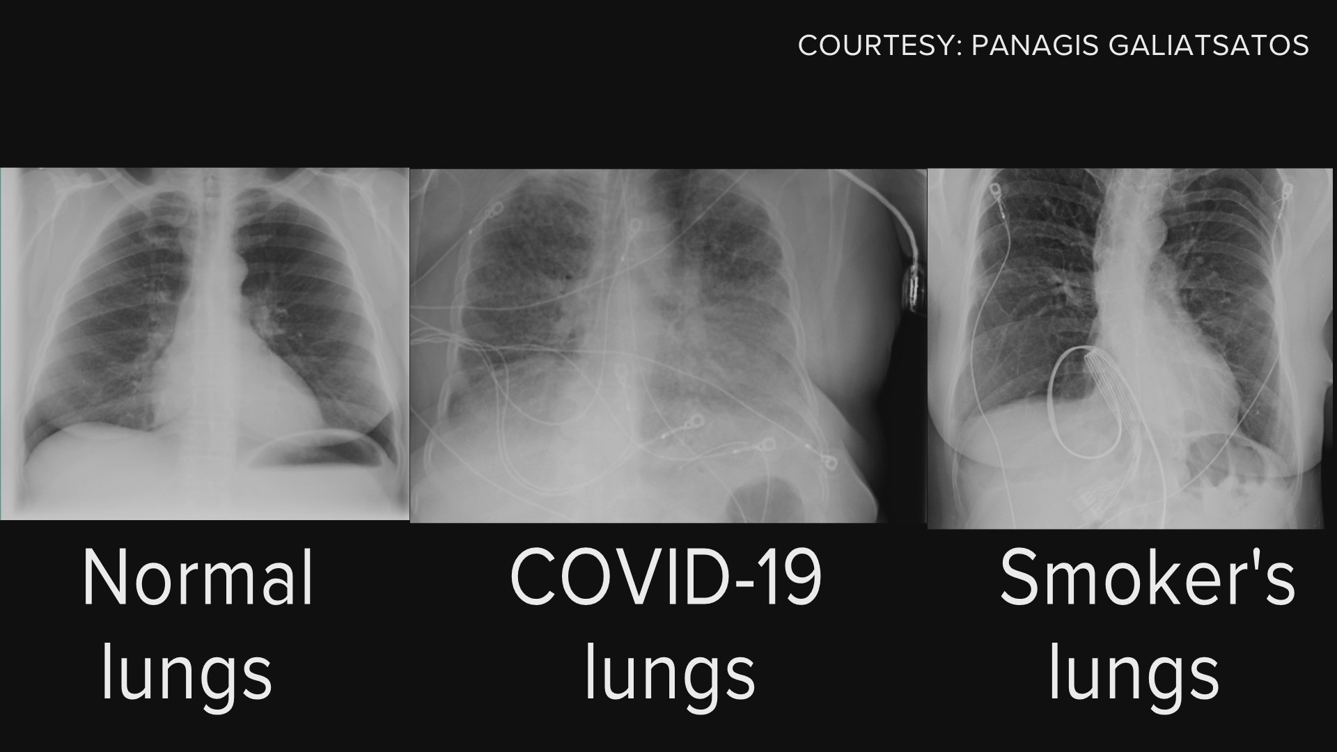
Normal vs. COVID vs. Smoking
The response \(Y\) in linear regression is numerical.
In many situations, \(Y\) is categorical!
A process of predicting categorical response is known as classification.
Regression Function \(f(x)\) vs. Classifier \(C(x)\)


Classification Example
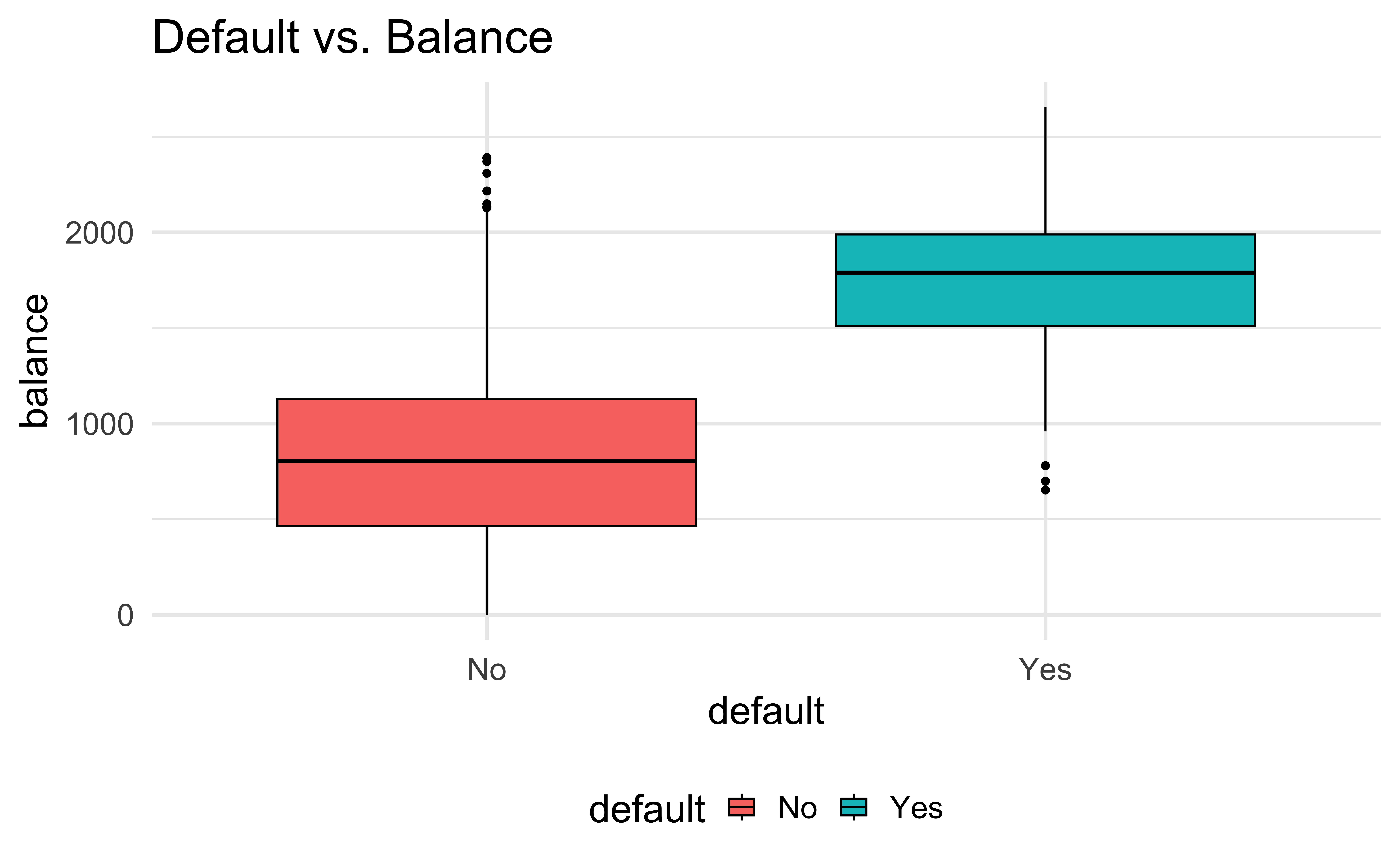
Predict whether people will default on their credit card payment \((Y)\)
yesorno, based on monthly credit card balance \((X)\).Use the training sample \(\{(x_1, y_1), \dots, (x_n, y_n)\}\) to build a classifier.

Binary Classification by Probability
Most of the time, we code categories using numbers! \(Y =\begin{cases} 0 & \quad \text{if not default}\\ 1 & \quad \text{if default} \end{cases}\)
First predict the probability of each category of \(Y\).
Predict probability of
defaultusing a S-shaped curve.

Binary Logistic Regression
Binary Responses with Nonconstant Probability
-
Training data \((x_1, y_1), \dots, (x_n, y_n)\) where
-
\(y_i = 1\) (
default) -
\(y_i = 0\) (
not default).
-
\(y_i = 1\) (
First predict \(P(y_i = 1 \mid x_i) = \pi(x_i) = \pi_i\)
The probability \(\pi\) changes with the value of predictor \(x\)!
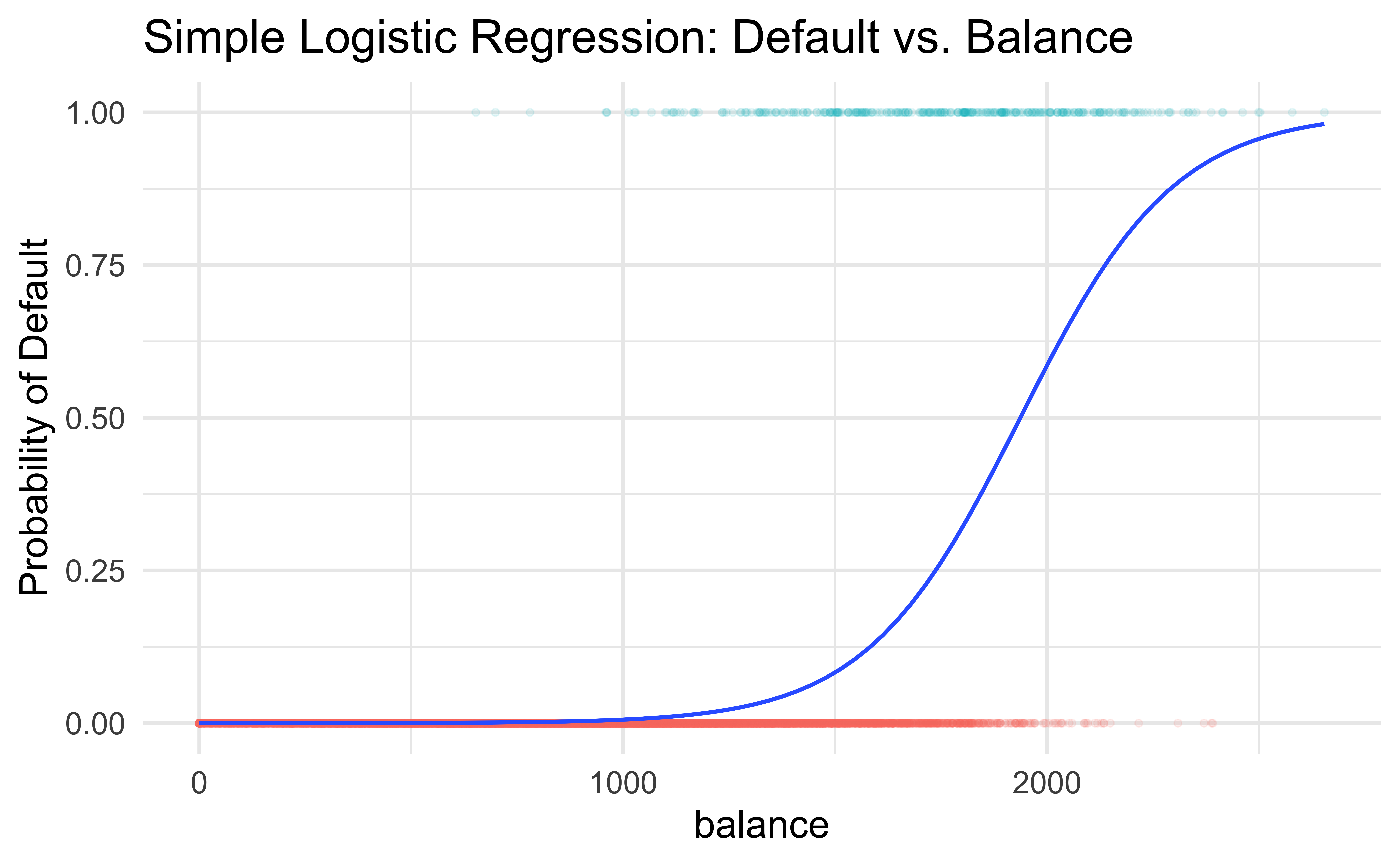
\(X =\)
balance. \(x_1 = 2000\) has a larger \(\pi_1 = \pi(2000)\) than \(\pi_2 = \pi(500)\) with \(x_2 = 500\).Credit cards with a higher balance is more likely to be default.
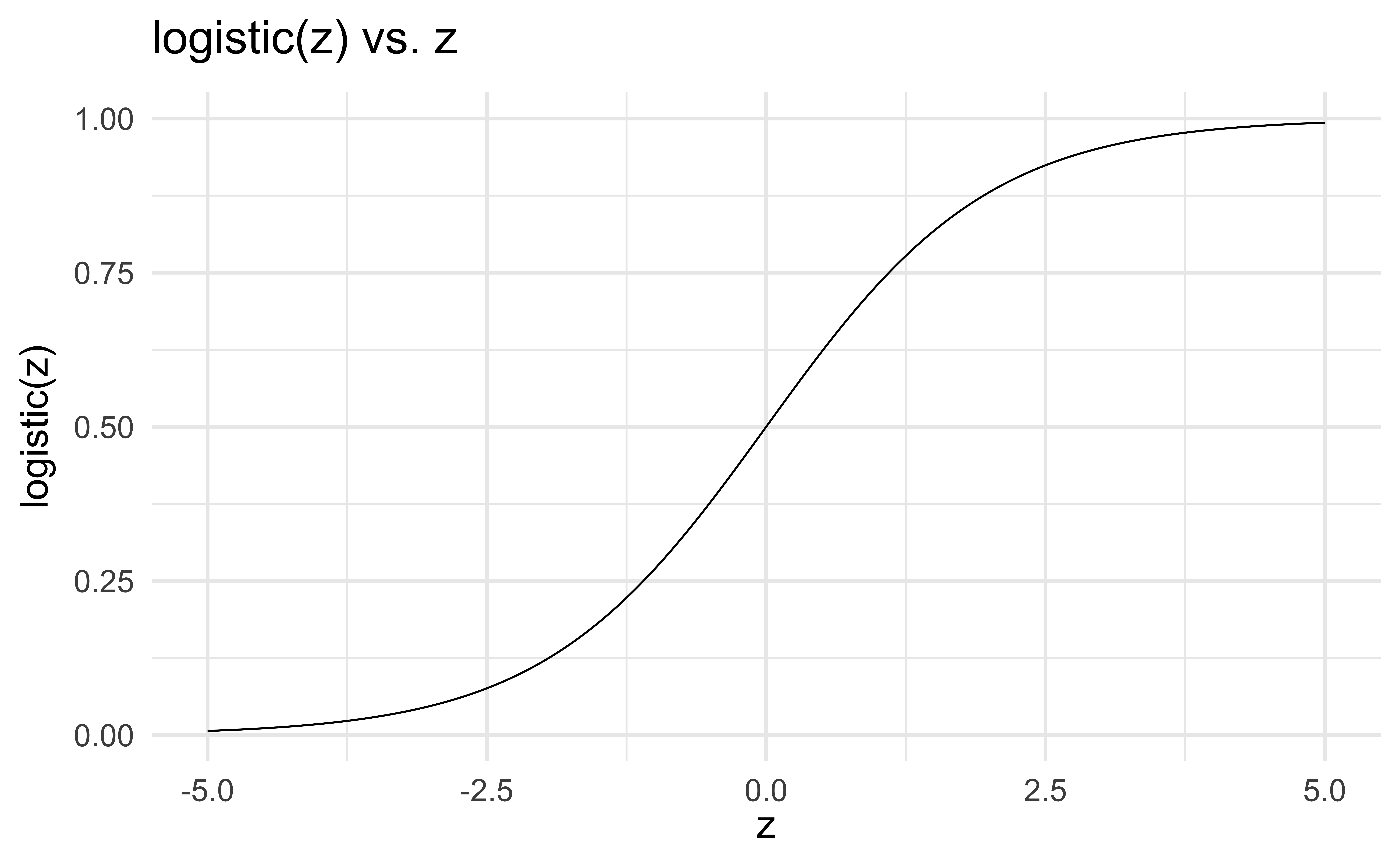
Logistic Function
- Assume \(\pi\) is affected by the linear function \(\beta_0 + \beta_1x\) with the logistic transformation:
\[\pi = \frac{1}{1+\exp(-(\beta_0 + \beta_1x))}\]
Does the logistic function guarantee that \(\pi \in (0, 1)\) for any value of \(\beta_0\), \(\beta_1\), and \(x\)?
Logistic Function \(\pi = \text{logistic}(\beta_0 + \beta_1x) = \frac{\exp(\beta_0 + \beta_1 x)}{1+\exp(\beta_0 + \beta_1 x)}\)
Simple Binary Logistic Regression Model
For \(i = 1, \dots, n\), and with one predictor \(X\): \[(Y_i \mid X = x_i) = \begin{cases} 1 & \quad \text{w/ prob } \pi(x_i)\\ 0 & \quad \text{w/ prob } 1 - \pi(x_i) \end{cases}\]
\[\pi(x_i) = \frac{1}{1+\exp(-(\beta_0+\beta_1 x_{i}))}\]
Goal: Get estimates \(\hat{\beta}_0\) and \(\hat{\beta}_1\), and therefore \(\hat{\pi}\)!
\[\small \hat{\pi} = \frac{1}{1+\exp(-\hat{\beta}_0-\hat{\beta}_1 x_{})}\]
Probability Curve
- The relationship between \(\pi(x)\) and \(x\) is not linear! \[\pi(x) = \frac{1}{1+\exp(-\beta_0-\beta_1 x)}\]
- The amount that \(\pi(x)\) changes due to a one-unit change in \(x\) depends on the current value of \(x\).
- Regardless of the value of \(x\), if \(\beta_1 > 0\), increasing \(x\) will be increasing \(\pi(x)\).

Fit Logistic Regression
bodydata <- read_csv("./data/body.csv")
body <- bodydata |>
    select(GENDER, HEIGHT) |>
    mutate(GENDER = as.factor(GENDER))
body |> slice(1:4)
# A tibble: 4 × 2
GENDER HEIGHT
<fct> <dbl>
1 0 172
2 1 186
3 0 154.
4 1 160.GENDER = 1if MaleGENDER = 0if FemaleUse
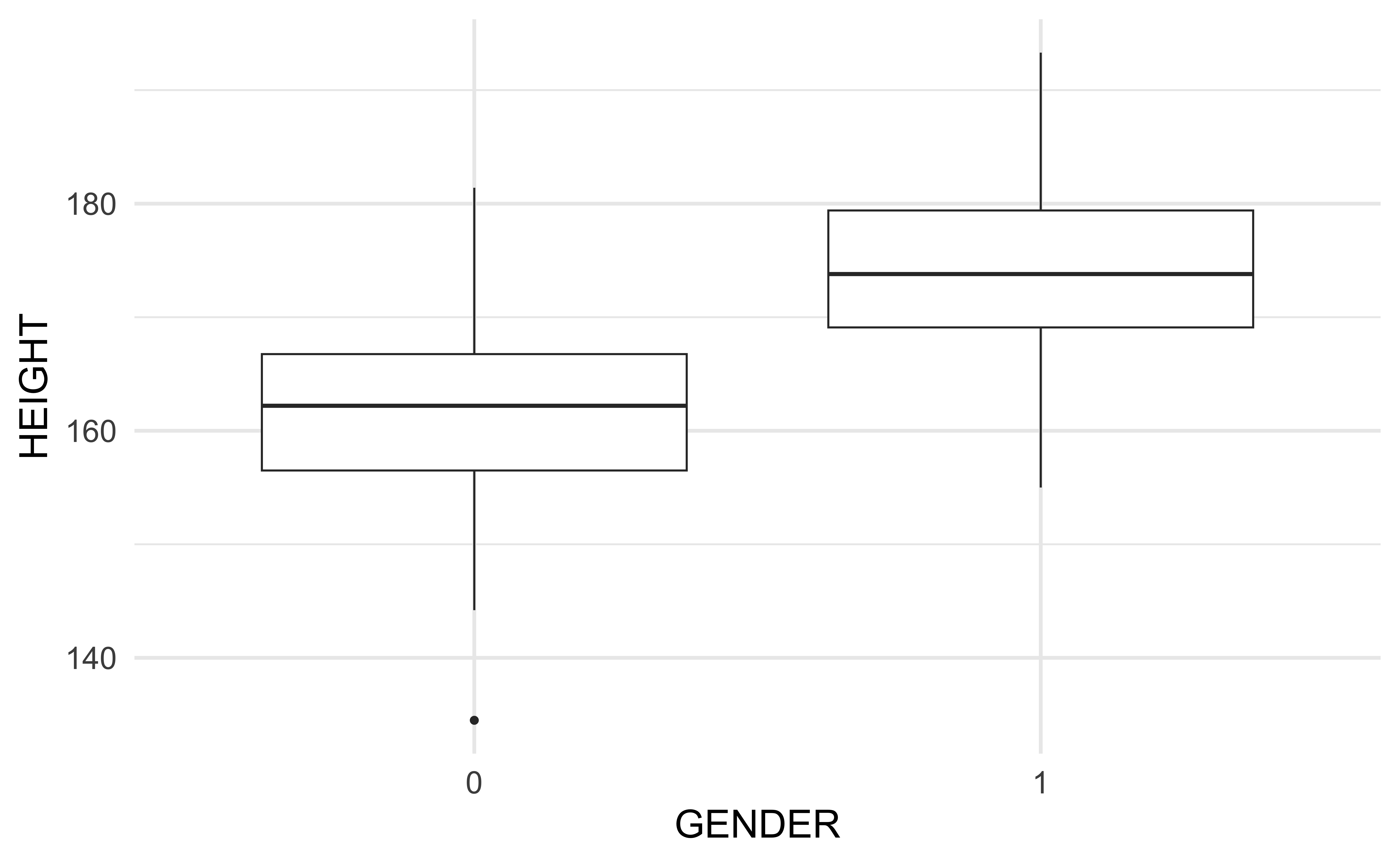
HEIGHT(centimeter, 1 cm = 0.39 in) to predict/classifyGENDER: whether one is male or female.

Logistic Regression - Data Summary
Logistic Regression - Model Fitting
Logistic Regression - Model Fitting
- Define
family = "binomial"
Probability Curve
     1      2      3      4      5      6
0.7369 0.9880 0.0383 0.1480 0.9383 0.4375 [1] 172 186 154 160 179 167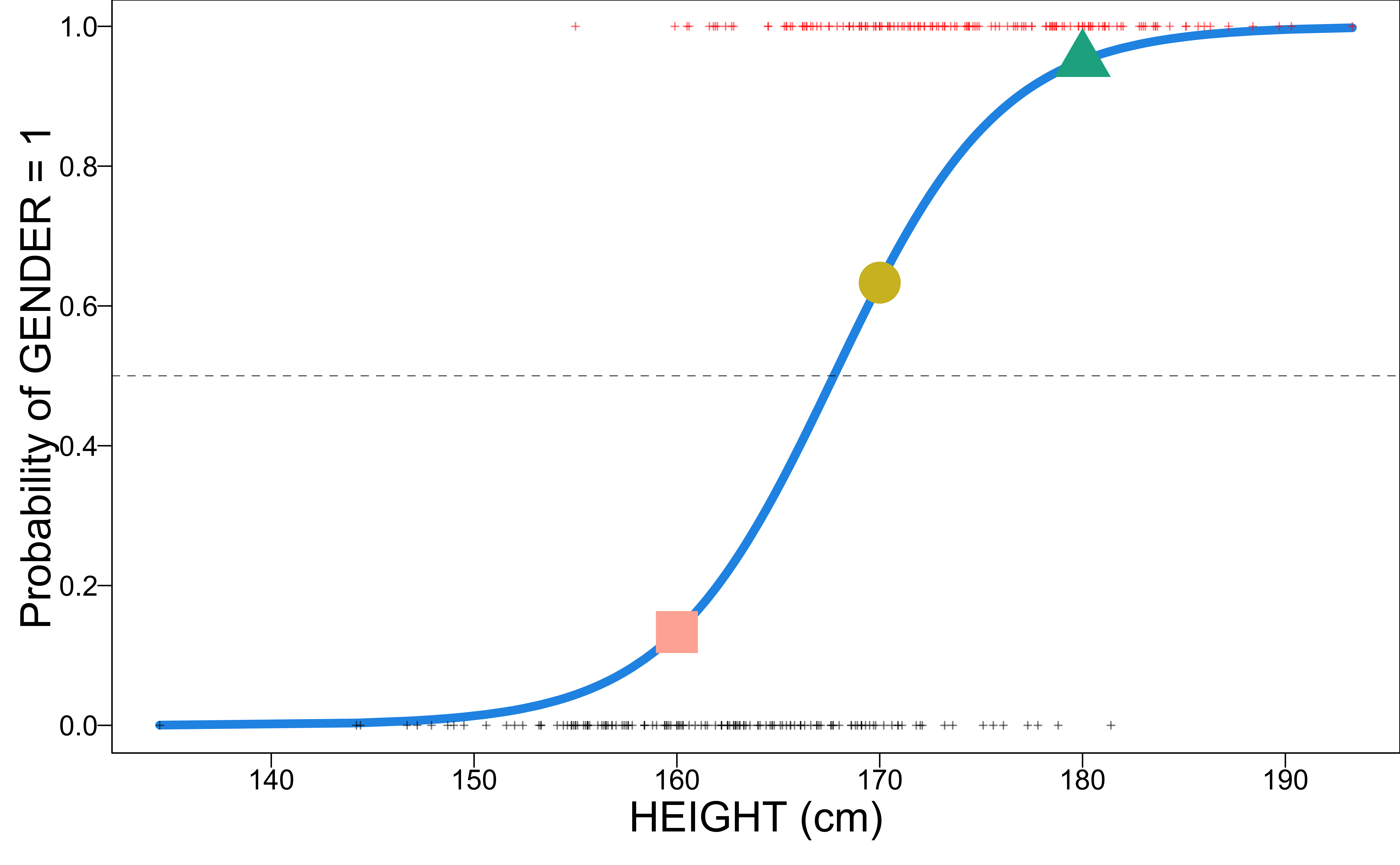
- 160 cm, Pr(male) = 0.13
- 170 cm, Pr(male) = 0.63
- 180 cm, Pr(male) = 0.95
21-Logistic Regression
In lab.qmd ## Lab 21 section,
Use our fitted logistic regression model to predict whether you are male or female! Change
175to your height (cm).Use the converter to get your height in cm!
sklearn.linear_model
sklearn.linear_model.LogisticRegression
sklearn.linear_model.LogisticRegression
array([[0.24154889]])array([-40.51727266])Evaluation
Evaluation Metrics1
- Confusion Matrix
| True 0 | True 1 | |
|---|---|---|
| Predict 0 | True Negative (TN) | False Negative (FN) |
| Predict 1 | False Positive (FP) | True Positive (TP) |
Sensitivity (True Positive Rate) \(= P( \text{predict 1} \mid \text{true 1}) = \frac{TP}{TP+FN}\)
Specificity (True Negative Rate) \(= P( \text{predict 0} \mid \text{true 0}) = \frac{TN}{FP+TN}\)
Accuracy \(= \frac{TP + TN}{TP+FN+FP+TN}\)
Confusion Matrix
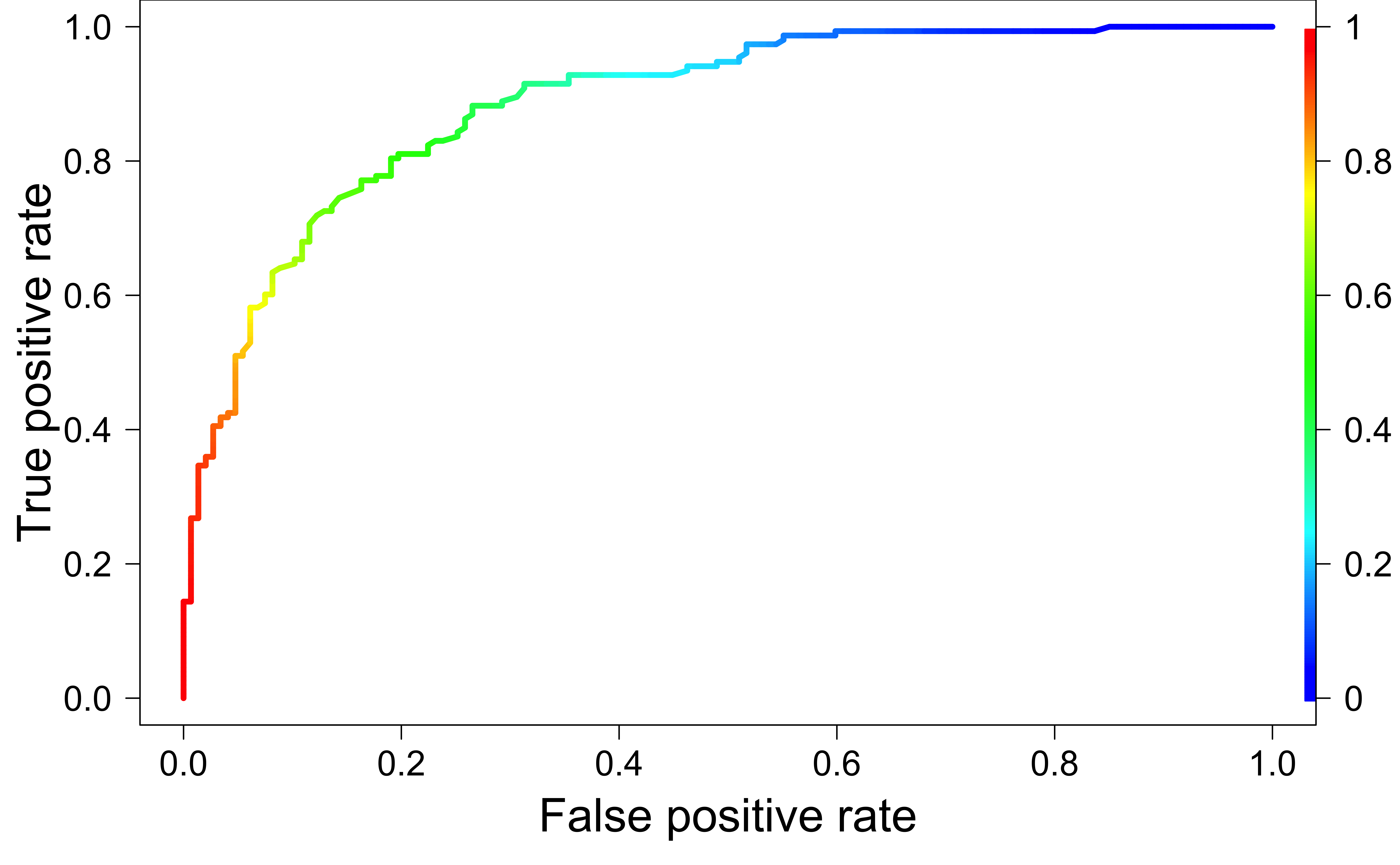
Receiver Operating Characteristic (ROC) Curve
| True 0 | True 1 | |
|---|---|---|
| Predict 0 | True Negative (TN) | False Negative (FN) |
| Predict 1 | False Positive (FP) | True Positive (TP) |
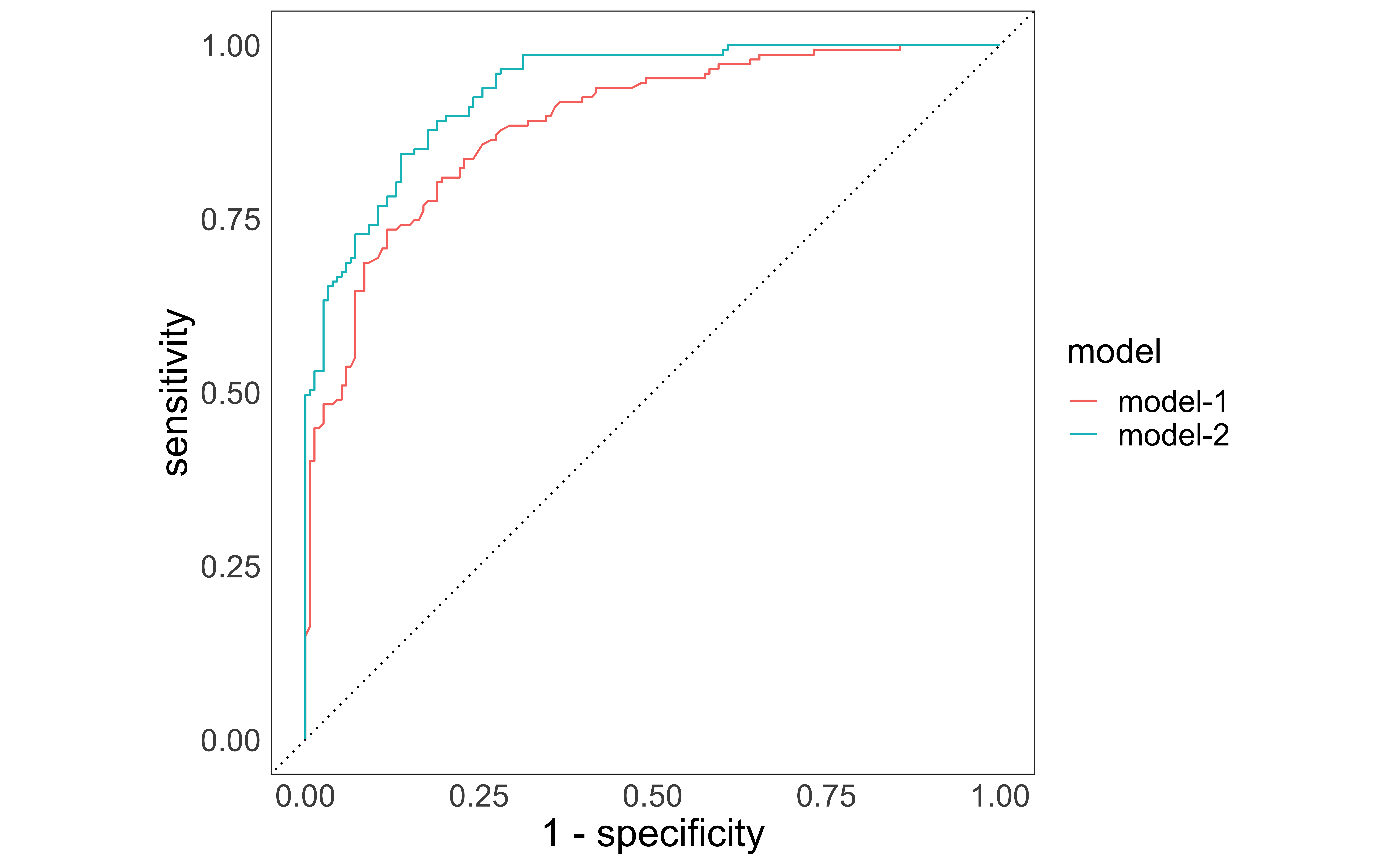
- Receiver operating characteristic (ROC) curve plots True Positive Rate (Sensitivity) vs. False Positive Rate (1 - Specificity)
Comparing Models
Which model performs better?
